Multi-species occupancy models

Fit a community (multi-species) occupancy model in base R with a hand-coded Gibbs sampler, and watch partial pooling stabilise sparse-species estimates.

When you survey a whole assemblage, most species are rare. A handful turn up almost everywhere; the long tail is seen at a few sites, on a few visits. Fit an occupancy model to each species on its own and the common ones behave, but the sparse ones fall apart: the likelihood has almost nothing to work with, and occupancy and detection trade off until the estimate lands on a boundary.

A community occupancy model treats the species as draws from a shared distribution. Each species keeps its own occupancy and detection probability, but those probabilities are tied together by community-level means and spreads. The rare species then borrow strength from the assemblage instead of standing alone. This tutorial builds the model from scratch in base R, samples it with a short Metropolis-within-Gibbs routine, and compares the pooled estimates against fitting every species separately.

A community with a long rare tail

We simulate 32 species across 90 sites, each visited 4 times. Species-level occupancy and detection are drawn on the logit scale from community distributions, so a few species are genuinely widespread and many are scarce.

library(ggplot2); library(dplyr); library(tidyr)
logit <- qlogis; expit <- plogis

# brand palette + theme
te_ink<-"#16241d"; te_body<-"#2c3a31"; te_forest<-"#275139"; te_faint<-"#5d6b61"
te_sage<-"#93a87f"; te_paper<-"#f5f4ee"; te_line<-"#dad9ca"; te_brick<-"#b5534e"
theme_te <- function(base_size=12){
  theme_minimal(base_size=base_size) +
    theme(plot.background=element_rect(fill=te_paper,colour=NA),
          panel.background=element_rect(fill="#ffffff",colour=NA),
          panel.grid.minor=element_blank(),
          panel.grid.major=element_line(colour=te_line,linewidth=0.3),
          axis.title=element_text(colour=te_body), axis.text=element_text(colour=te_faint),
          plot.title=element_text(colour=te_ink,face="bold"),
          plot.subtitle=element_text(colour=te_faint,size=rel(0.9)),
          legend.text=element_text(colour=te_faint,size=rel(0.8)))
}

set.seed(143)
S <- 32L; R <- 90L; K <- 4L                 # species, sites, visits
mu_lpsi <- logit(0.40); sd_lpsi <- 1.30     # community occupancy (logit scale)
mu_lp   <- logit(0.27); sd_lp   <- 0.95     # community detection (logit scale)

lpsi_t <- rnorm(S, mu_lpsi, sd_lpsi)        # true species occupancy logits
lp_t   <- rnorm(S, mu_lp,   sd_lp)          # true species detection logits
psi_t  <- expit(lpsi_t); p_t <- expit(lp_t)

z_t <- matrix(rbinom(S*R, 1, psi_t), nrow=S, ncol=R)          # occupancy state
y   <- matrix(rbinom(S*R, K, ifelse(z_t==1, p_t, 0)), S, R)   # detection counts
det_sites <- rowSums(y > 0)                                    # sites each species was seen at

Detection frequencies run from 2 to 80 sites, and 7 species were detected at fewer than ten sites. Every species was seen at least once here; the separate problem of species that are never detected is taken up in estimating species richness with data augmentation.

Fitting every species on its own

The single-season occupancy likelihood collapses over the unknown occupancy state at each site: a site with a detection must be occupied, and a site with no detection is either unoccupied or occupied but missed. We maximise that likelihood species by species.

nll_ss <- function(par, yi){
  psi <- expit(par[1]); p <- expit(par[2]); det <- yi > 0
  ll <- sum(log(psi) + dbinom(yi[det], K, p, log=TRUE)) +
        sum((!det) * log(psi*(1-p)^K + (1-psi)))
  -ll
}
ss_psi <- ss_p <- rep(NA_real_, S); boundary <- logical(S)
for (s in 1:S){
  op <- optim(c(0,0), nll_ss, yi=y[s,], method="BFGS")
  ss_psi[s] <- expit(op$par[1]); ss_p[s] <- expit(op$par[2])
  boundary[s] <- ss_psi[s]>0.995 || ss_psi[s]<0.005 || ss_p[s]>0.995 || ss_p[s]<0.005
}
sum(boundary)   # species whose independent estimate is pinned at a boundary

[1] 5

5 of the 32 species land on a boundary of the parameter space. The two rarest, each detected at just 2 sites, illustrate why: their independent occupancy estimates are 0.98 and 0.98 with detection estimates near zero, which is the likelihood giving up rather than a real result.

The community model

Give species s an occupancy logit lpsi[s] and a detection logit lp[s], and let those come from community distributions with means mu_psi, mu_p and standard deviations sd_psi, sd_p. We sample the whole set with random-walk Metropolis updates for the species effects and the hyperparameters, marginalising the occupancy state analytically so there is no latent matrix to carry.

ni <- 18000L; nb <- 6000L; nt <- 3L
lpsi <- logit(pmin(pmax((det_sites+0.5)/(R+1), 0.02), 0.98)); lp <- rep(logit(0.3), S)
mps <- 0; sps <- 1; mp <- logit(0.3); sp <- 1               # hyperparameters
t_lpsi<-0.30; t_lp<-0.26; t_mu<-0.14; t_lsd<-0.14           # proposal scales
keep <- seq(nb+1, ni, by=nt); nk <- length(keep)
PSI <- matrix(NA,nk,S); P <- matrix(NA,nk,S); HYP <- matrix(NA,nk,4); kk <- 0L

for (it in 1:ni){
  psi <- expit(lpsi); p <- expit(lp)
  # sum of occupied sites, drawing the latent state at undetected sites (Gibbs)
  pz <- psi*(1-p)^K / (psi*(1-p)^K + (1-psi))
  z  <- ifelse(y==0, matrix(rbinom(S*R,1,pz),S,R), 1L); sumz <- rowSums(z)
  # species occupancy logits (Metropolis)
  prop <- lpsi + rnorm(S,0,t_lpsi); psip <- expit(prop)
  a <- sumz*log(psip)+(R-sumz)*log(1-psip)+dnorm(prop,mps,sps,log=TRUE) -
       (sumz*log(psi)+(R-sumz)*log(1-psi)+dnorm(lpsi,mps,sps,log=TRUE))
  au <- log(runif(S)) < a; lpsi[au] <- prop[au]
  # species detection logits (Metropolis), over occupied sites
  p <- expit(lp); occ <- z==1; Sy <- rowSums(y*occ); SKy <- rowSums((K-y)*occ)
  prop <- lp + rnorm(S,0,t_lp); pp <- expit(prop)
  a <- Sy*log(pp)+SKy*log(1-pp)+dnorm(prop,mp,sp,log=TRUE) -
       (Sy*log(p)+SKy*log(1-p)+dnorm(lp,mp,sp,log=TRUE))
  au <- log(runif(S)) < a; lp[au] <- prop[au]
  # community means and spreads (Metropolis; half-normal prior on the spreads)
  pr <- mps+rnorm(1,0,t_mu)
  if (log(runif(1)) < sum(dnorm(lpsi,pr,sps,log=TRUE))-sum(dnorm(lpsi,mps,sps,log=TRUE))) mps <- pr
  pr <- exp(log(sps)+rnorm(1,0,t_lsd))
  if (log(runif(1)) < sum(dnorm(lpsi,mps,pr,log=TRUE))+dnorm(pr,0,2.5,log=TRUE)+log(pr)-
                      sum(dnorm(lpsi,mps,sps,log=TRUE))-dnorm(sps,0,2.5,log=TRUE)-log(sps)) sps <- pr
  pr <- mp+rnorm(1,0,t_mu)
  if (log(runif(1)) < sum(dnorm(lp,pr,sp,log=TRUE))-sum(dnorm(lp,mp,sp,log=TRUE))) mp <- pr
  pr <- exp(log(sp)+rnorm(1,0,t_lsd))
  if (log(runif(1)) < sum(dnorm(lp,mp,pr,log=TRUE))+dnorm(pr,0,2.5,log=TRUE)+log(pr)-
                      sum(dnorm(lp,mp,sp,log=TRUE))-dnorm(sp,0,2.5,log=TRUE)-log(sp)) sp <- pr
  if (it>nb && ((it-nb) %% nt == 0)){ kk<-kk+1L
    PSI[kk,]<-expit(lpsi); P[kk,]<-expit(lp); HYP[kk,]<-c(mps,sps,mp,sp) }
}
comm_psi <- colMeans(PSI); hyp <- colMeans(HYP)
c(community_occupancy = round(expit(hyp[1]),3), community_detection = round(expit(hyp[3]),3))

community_occupancy community_detection 
              0.514               0.280 

The community mean occupancy is 0.514, close to the assemblage average of 0.494 that generated the data. The among-species spread is harder to pin down: the posterior for the occupancy standard deviation runs from 1.45 to 2.73 on the logit scale. Estimating that spread from imperfect detections is a genuinely difficult part of the problem, so wide intervals here are honest rather than a fault.

Pooling in action

The payoff is at the sparse end. Species with few detections have independent estimates scattered from near zero to near one; the community model pulls them back toward the assemblage, where the evidence actually points.

comm_mean <- expit(hyp[1])
df  <- data.frame(det=det_sites, ind=ss_psi, comm=comm_psi)
seg <- data.frame(det=df$det, y1=df$ind, y2=df$comm)
ggplot() +
  geom_hline(yintercept=comm_mean, linetype="dashed", colour=te_faint) +
  geom_segment(data=seg, aes(det, y1, xend=det, yend=y2), colour=te_sage, linewidth=0.4) +
  geom_point(data=df, aes(det, ind, shape="Independent (per species)"), colour=te_brick, size=2) +
  geom_point(data=df, aes(det, comm, shape="Community (pooled)"), colour=te_forest, size=2) +
  scale_shape_manual(NULL, values=c("Independent (per species)"=1,"Community (pooled)"=16)) +
  scale_x_continuous(trans="sqrt", breaks=c(2,5,10,20,40,80)) +
  labs(x="sites where the species was detected (sqrt scale)", y="occupancy estimate (psi)",
       title="Rare-species estimates are pulled toward the community",
       subtitle="dashed line: community mean; segments join the two estimates for each species") +
  theme_te() + theme(legend.position=c(0.75,0.15),
                     legend.background=element_rect(fill="#ffffff",colour=te_line))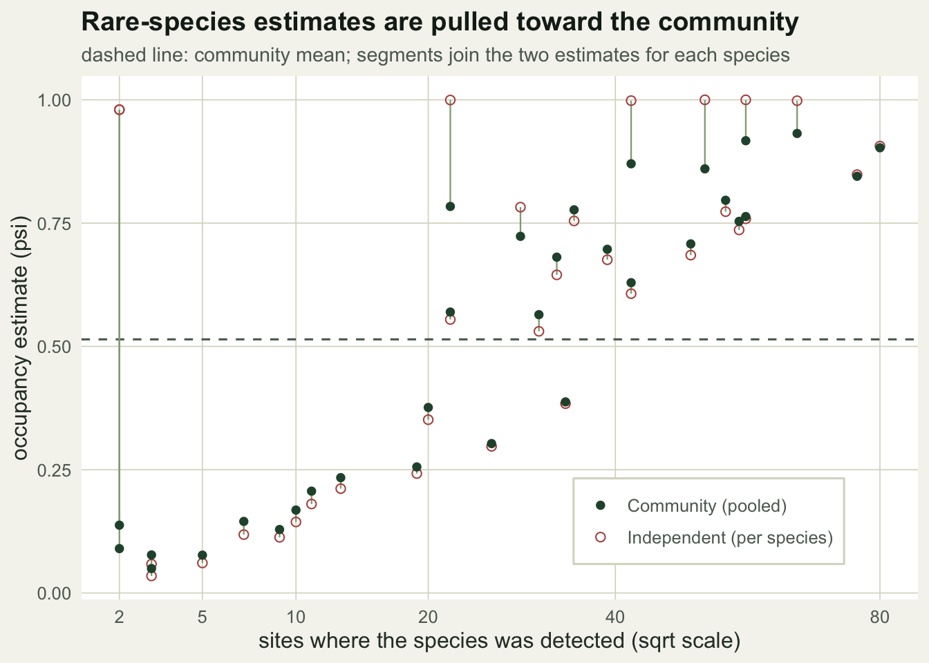

Figure 1: Occupancy estimates against detection frequency, fitted per species and pooled across the community.

Averaged over all species, the pooled estimates sit closer to the truth: the mean absolute error in occupancy falls from 0.125 for the independent fits to 0.067 for the community model. The estimates are also less scattered, with a spread of 0.311 against 0.341, because the extreme boundary values have been reined in.

The model also reports the distribution of species itself. The fitted community is right-skewed, with many low-occupancy species and a thin high-occupancy tail, and the per-species estimates sit underneath it.

xx <- seq(-6, 5, length=400)
dens <- data.frame(psi=expit(xx)); lp_ax <- logit(dens$psi)
dens$dp <- dnorm(lp_ax, hyp[1], hyp[2]) / (dens$psi*(1-dens$psi))    # change of variable to psi scale
sp <- data.frame(psi=comm_psi)
ggplot() +
  geom_area(data=subset(dens, psi>1e-3 & psi<0.999), aes(psi, dp), fill=te_sage, alpha=0.35) +
  geom_line(data=subset(dens, psi>1e-3 & psi<0.999), aes(psi, dp), colour=te_forest, linewidth=0.7) +
  geom_rug(data=sp, aes(psi), colour=te_brick, length=unit(0.05,"npc")) +
  geom_point(data=sp, aes(psi, y=0), colour=te_brick, size=1.6, alpha=0.8) +
  labs(x="species occupancy (psi)", y="community density",
       title="The estimated distribution of species occupancy",
       subtitle="curve: fitted community (logit-normal); ticks: per-species posterior means") +
  theme_te()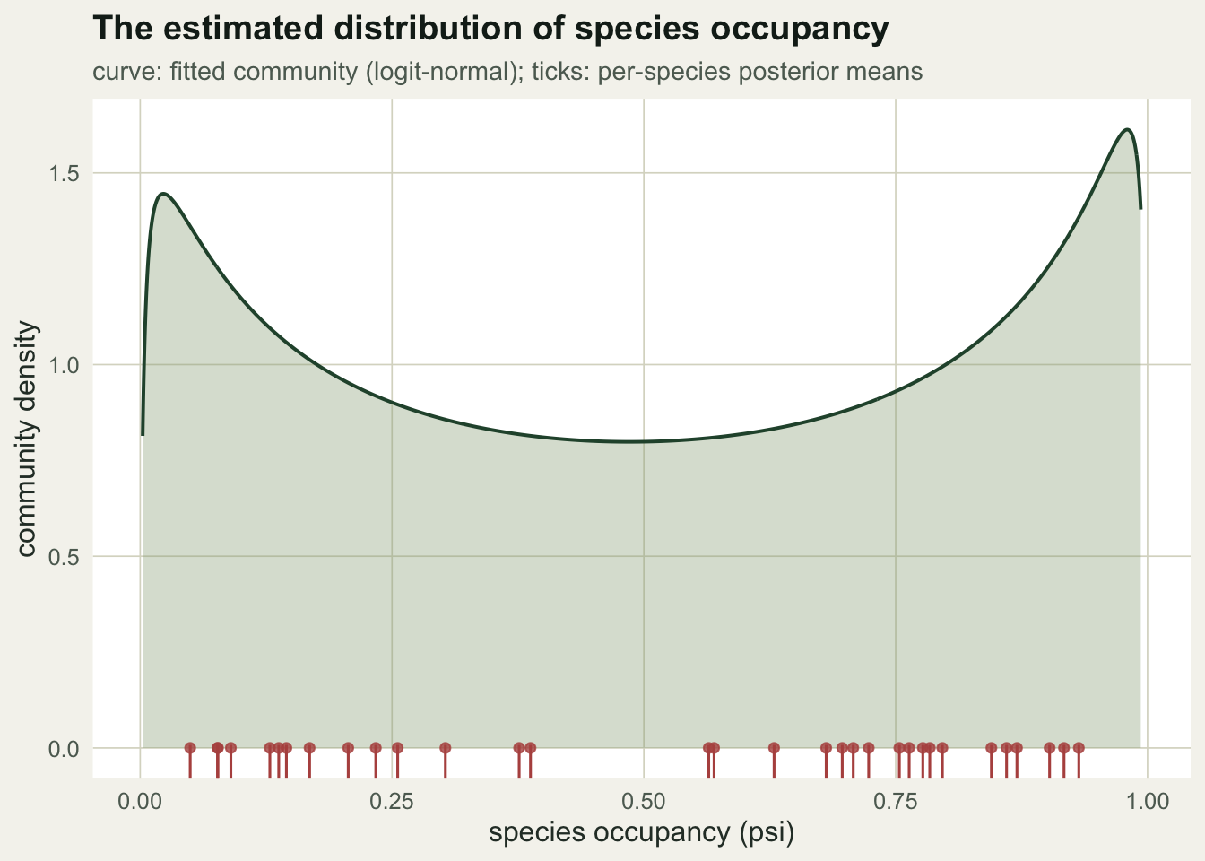

Figure 2: The fitted community distribution of occupancy, with per-species posterior means beneath it.

What the pooling does and does not do

Partial pooling is a compromise, not a free lunch. It moves sparse-species estimates toward the community mean in proportion to how little each species tells us on its own, which reduces error on average but shrinks a genuinely unusual rare species toward the crowd. The assumption that species are exchangeable draws from one distribution is doing real work; if the assemblage is really two guilds with very different occupancy, a single community distribution will misrepresent both, and that is worth checking (see checking a community occupancy model).

The community mean and the species-level estimates are recovered well; the among-species variance is not, and that is the usual pattern with imperfect detection. From here you can add site covariates with species-specific responses and let a trait explain the variation among species, which is the subject of community covariates and species traits.

Related tutorials

• Estimating species richness with data augmentation
• Community covariates and species traits
• Checking a community occupancy model
• Single-season occupancy model

References

• Dorazio & Royle 2005 Journal of the American Statistical Association 100(470):389-398 (10.1198/016214505000000015)
• Dorazio, Royle, Soderstrom & Glimskar 2006 Ecology 87(4):842-854 (10.1890/0012-9658(2006)87[842:ESRAAB]2.0.CO;2)
• Kery & Royle 2008 Journal of Applied Ecology 45(2):589-598 (10.1111/j.1365-2664.2007.01441.x)
• Zipkin, DeWan & Royle 2009 Journal of Applied Ecology 46(4):815-822 (10.1111/j.1365-2664.2009.01664.x)
• Gelman, Meng & Stern 1996 Statistica Sinica 6(4):733-807
• Kery & Royle 2016. Applied Hierarchical Modeling in Ecology, Volume 1. Academic Press. ISBN 978-0-12-801378-6
• Royle & Dorazio 2008. Hierarchical Modeling and Inference in Ecology. Academic Press. ISBN 978-0-12-374097-7