library(ggplot2); library(dplyr)
logit <- qlogis; expit <- plogis

te_ink<-"#16241d"; te_body<-"#2c3a31"; te_forest<-"#275139"; te_faint<-"#5d6b61"
te_sage<-"#93a87f"; te_paper<-"#f5f4ee"; te_line<-"#dad9ca"; te_brick<-"#b5534e"; te_gold<-"#cda23f"
theme_te <- function(base_size=12){
  theme_minimal(base_size=base_size) +
    theme(plot.background=element_rect(fill=te_paper,colour=NA),
          panel.background=element_rect(fill="#f5f4ee",colour=NA),
          panel.grid.minor=element_blank(),
          panel.grid.major=element_line(colour=te_line,linewidth=0.3),
          axis.title=element_text(colour=te_body), axis.text=element_text(colour=te_faint),
          plot.title=element_text(colour=te_ink,face="bold"),
          plot.subtitle=element_text(colour=te_faint,size=rel(0.9)),
          legend.text=element_text(colour=te_faint,size=rel(0.8)))
}Community covariates and species traits
ecology tutorial
R
occupancy
hierarchical models
Bayesian statistics
MCMC
community ecology
Give each species its own slope on a site gradient, and use a trait to explain the variation. A hierarchical model in base R, set against the two-stage fit.
Corrected 27 September 2026: the post said the independent slopes are noisiest for the rarely detected species; the figure shows the largest departures among moderately and well-detected species, and the text now says so.
Species do not all respond to an environmental gradient the same way. Some occupy more sites as the gradient increases; others retreat. A community occupancy model can give every species its own slope on a site covariate, and then ask whether a species trait explains why the slopes differ. That second step is the interesting one: it turns a pile of species-specific responses into a statement about how a trait shapes the response.
The tempting shortcut is to fit each species on its own, collect the slope estimates, and regress them on the trait. That two-stage approach ignores how noisy the per-species slopes are, and some of them are barely identified by the data at all. This tutorial builds the integrated hierarchical model in base R, and sets it against the two-stage shortcut.
A gradient, a trait, and species-specific slopes
We simulate 34 species across 95 sites with 4 visits. Occupancy of species s at site r depends on a standardised site covariate through a species-specific intercept and slope. Each species slope is itself drawn around a line in the species trait, so the trait genuinely drives the response.
set.seed(145)
S <- 34L; R <- 95L; K <- 4L
x  <- as.numeric(scale(rnorm(R)))          # site covariate (standardised)
tr <- as.numeric(scale(rnorm(S)))          # species trait (standardised)
mu_a <- logit(0.35); sd_a <- 0.85          # community intercept
beta0 <- 0.20; beta1 <- 0.90; sd_b <- 0.50 # slope depends on trait: b ~ N(beta0 + beta1*tr, sd_b)
mu_p <- logit(0.30); sd_p <- 0.60          # community detection

a_t <- rnorm(S, mu_a, sd_a)                          # species intercepts
b_t <- rnorm(S, beta0 + beta1*tr, sd_b)              # species slopes, tied to the trait
lp_t <- rnorm(S, mu_p, sd_p); p_t <- expit(lp_t)
eta <- matrix(a_t, S, R) + outer(b_t, x); psi <- expit(eta)
z <- matrix(rbinom(S*R, 1, psi), S, R)
y <- matrix(rbinom(S*R, K, ifelse(z==1, p_t, 0)), S, R)
det_sites <- rowSums(y > 0)
c(species=S, sites=R, det_min=min(det_sites), det_max=max(det_sites), total_det=sum(y))
species sites det_min det_max total_det
34 95 6 56 1545 Detection frequencies run from 6 to 56 sites. That range matters, although, as the slope figure below shows, a small detection count is not the only thing that leaves a slope poorly identified on its own.
Independent slopes, and why they mislead
Fit each species with its own occupancy-covariate model (as in occupancy with detection covariates), pulling the slope and its standard error from the Hessian.
one <- function(yi){
  nll <- function(par){ a<-par[1]; b<-par[2]; p<-expit(par[3]); ps<-expit(a+b*x); d<-yi>0
    -(sum(log(ps[d]) + dbinom(yi[d],K,p,log=TRUE)) + sum(log(ps[!d]*(1-p)^K + (1-ps[!d])))) }
  op <- try(optim(c(logit(mean(yi>0)+.01),0,0), nll, method="BFGS", hessian=TRUE), silent=TRUE)
  if (inherits(op,"try-error")) return(c(b=NA, se=NA))
  se <- try(sqrt(diag(solve(op$hessian)))[2], silent=TRUE)
  c(b=op$par[2], se=ifelse(inherits(se,"try-error")||is.na(se), NA, se))
}
mle <- t(sapply(1:S, function(s) one(y[s,]))); colnames(mle) <- c("b","se")
round(c(median_SE=median(mle[,"se"]), max_SE=max(mle[,"se"])), 2)
median_SE max_SE
0.36 4.82 The chunk above prints the median and the largest of the per-species standard errors. A species detected at only a handful of sites carries little information about its own slope, and a fit like that can return no usable standard error at all. Now take the tempting shortcut and regress the per-species slopes on the trait.
ok <- is.finite(mle[,"b"]) & is.finite(mle[,"se"])   # drop any species without a finite estimate
naive <- lm(mle[ok,"b"] ~ tr[ok])
c(beta1_naive = round(coef(naive)[2],3), true = beta1)
beta1_naive.tr[ok] true
1.482 0.900 The naive two-stage slope is 1.482; the true value is 0.9. Regressing point estimates while ignoring their very unequal precision gives a species with a barely identified slope the same weight as one estimated from plenty of detections.
The integrated hierarchical model
Fit everything at once. Species intercepts come from a community distribution; species slopes come from a line in the trait; detection has its own community distribution. The occupancy state is summed out site by site, and every continuous parameter is updated with random-walk Metropolis.
llmat <- function(a, b, lp){                       # per-species log-likelihood, z summed out
  e <- matrix(a,S,R) + outer(b,x); ps <- expit(e); p <- expit(lp); Pm <- matrix(p,S,R)
  D <- y>0; term <- matrix(0,S,R)
  term[D]  <- log(ps[D]) + dbinom(y[D],K,Pm[D],log=TRUE)
  term[!D] <- log(ps[!D]*(1-Pm[!D])^K + (1-ps[!D]))
  rowSums(term)
}
ni <- 16000L; nb <- 6000L; nt <- 2L
a <- rep(logit(0.35),S); b <- rep(0,S); lp <- rep(logit(0.3),S)
m_a<-0; s_a<-1; B0<-0; B1<-0; s_b<-1; m_p<-logit(0.3); s_p<-1
t_a<-0.22; t_b<-0.22; t_lp<-0.22; t_h<-0.13; t_lsd<-0.13
keep <- seq(nb+1,ni,by=nt); nk <- length(keep); kk <- 0L
Bpost <- matrix(NA,nk,S); HYP <- matrix(NA,nk,7)    # m_a,s_a,B0,B1,s_b,m_p,s_p

for (it in 1:ni){
  ll <- llmat(a,b,lp)
  prop <- a + rnorm(S,0,t_a); llp <- llmat(prop,b,lp)                    # intercepts
  au <- log(runif(S)) < (llp+dnorm(prop,m_a,s_a,log=TRUE) - (ll+dnorm(a,m_a,s_a,log=TRUE))); a[au]<-prop[au]
  ll <- llmat(a,b,lp)
  mb <- B0 + B1*tr
  prop <- b + rnorm(S,0,t_b); llp <- llmat(a,prop,lp)                    # slopes (prior mean B0+B1*trait)
  au <- log(runif(S)) < (llp+dnorm(prop,mb,s_b,log=TRUE) - (ll+dnorm(b,mb,s_b,log=TRUE))); b[au]<-prop[au]
  ll <- llmat(a,b,lp)
  prop <- lp + rnorm(S,0,t_lp); llp <- llmat(a,b,prop)                   # detection
  au <- log(runif(S)) < (llp+dnorm(prop,m_p,s_p,log=TRUE) - (ll+dnorm(lp,m_p,s_p,log=TRUE))); lp[au]<-prop[au]
  # hyperparameters
  pr<-m_a+rnorm(1,0,t_h); if(log(runif(1))<sum(dnorm(a,pr,s_a,log=TRUE))-sum(dnorm(a,m_a,s_a,log=TRUE)))m_a<-pr
  pr<-exp(log(s_a)+rnorm(1,0,t_lsd)); if(log(runif(1))<sum(dnorm(a,m_a,pr,log=TRUE))+dnorm(pr,0,2.5,log=TRUE)+log(pr)-sum(dnorm(a,m_a,s_a,log=TRUE))-dnorm(s_a,0,2.5,log=TRUE)-log(s_a))s_a<-pr
  mb<-B0+B1*tr; pr<-B0+rnorm(1,0,t_h); if(log(runif(1))<sum(dnorm(b,pr+B1*tr,s_b,log=TRUE))-sum(dnorm(b,mb,s_b,log=TRUE)))B0<-pr
  mb<-B0+B1*tr; pr<-B1+rnorm(1,0,t_h); if(log(runif(1))<sum(dnorm(b,B0+pr*tr,s_b,log=TRUE))-sum(dnorm(b,mb,s_b,log=TRUE)))B1<-pr
  mb<-B0+B1*tr; pr<-exp(log(s_b)+rnorm(1,0,t_lsd)); if(log(runif(1))<sum(dnorm(b,mb,pr,log=TRUE))+dnorm(pr,0,2.5,log=TRUE)+log(pr)-sum(dnorm(b,mb,s_b,log=TRUE))-dnorm(s_b,0,2.5,log=TRUE)-log(s_b))s_b<-pr
  pr<-m_p+rnorm(1,0,t_h); if(log(runif(1))<sum(dnorm(lp,pr,s_p,log=TRUE))-sum(dnorm(lp,m_p,s_p,log=TRUE)))m_p<-pr
  pr<-exp(log(s_p)+rnorm(1,0,t_lsd)); if(log(runif(1))<sum(dnorm(lp,m_p,pr,log=TRUE))+dnorm(pr,0,2.5,log=TRUE)+log(pr)-sum(dnorm(lp,m_p,s_p,log=TRUE))-dnorm(s_p,0,2.5,log=TRUE)-log(s_p))s_p<-pr
  if (it>nb && ((it-nb)%%nt==0)){ kk<-kk+1L; Bpost[kk,]<-b; HYP[kk,]<-c(m_a,s_a,B0,B1,s_b,m_p,s_p) }
}
hp <- colMeans(HYP); bhat <- colMeans(Bpost)
round(c(beta0=hp[3], beta1=hp[4], sd_b=hp[5]), 3)
beta0 beta1 sd_b
0.288 0.928 0.439 The hierarchical trait effect is 0.928, with a 95 per cent interval from 0.71 to 1.17. That interval covers the true value of 0.9. The model also recovers the detection spread and the intercept spread reasonably, with a slope standard deviation of 0.44 around the trait line.
Pooling the slopes
The species slopes tell the story directly. Ordered by how often each species was detected, the independent estimates do not settle down at the well-detected end: the largest gaps between independent and pooled slopes, and the longest error bars, sit among the moderately and well-detected species, and one independent slope (rank 27) runs off the clipped scale altogether. The pooled slopes are pulled toward the community relationship wherever a species’ own estimate is poorly identified.
df <- data.frame(det=det_sites, mle=mle[,"b"], se=mle[,"se"], hier=bhat)
df <- df[order(df$det),]; df$rank <- 1:S; comm_mean <- mean(bhat)
ggplot(df, aes(rank)) +
  geom_hline(yintercept=comm_mean, linetype="dashed", colour=te_faint) +
  geom_errorbar(aes(ymin=mle-se, ymax=mle+se), colour=te_brick, width=0, linewidth=0.4, alpha=0.7) +
  geom_point(aes(y=mle, shape="Independent (per species) +/-1 SE"), colour=te_brick, size=1.7) +
  geom_point(aes(y=hier, shape="Hierarchical (partially pooled)"), colour=te_forest, size=1.7) +
  scale_shape_manual(NULL, values=c("Independent (per species) +/-1 SE"=1,"Hierarchical (partially pooled)"=16)) +
  coord_cartesian(ylim=c(-4,4)) +
  labs(x="species ordered by number of detections (fewest at left)", y="occupancy-covariate slope",
       title="Ill-identified slopes are noisy; pooling reins them in",
       subtitle="dashed: community mean; the vertical scale is clipped at plus and minus 4") +
  theme_te() + theme(legend.position = "inside", legend.position.inside = c(0.72,0.13),
                     legend.background=element_rect(fill="#ffffff",colour=te_line))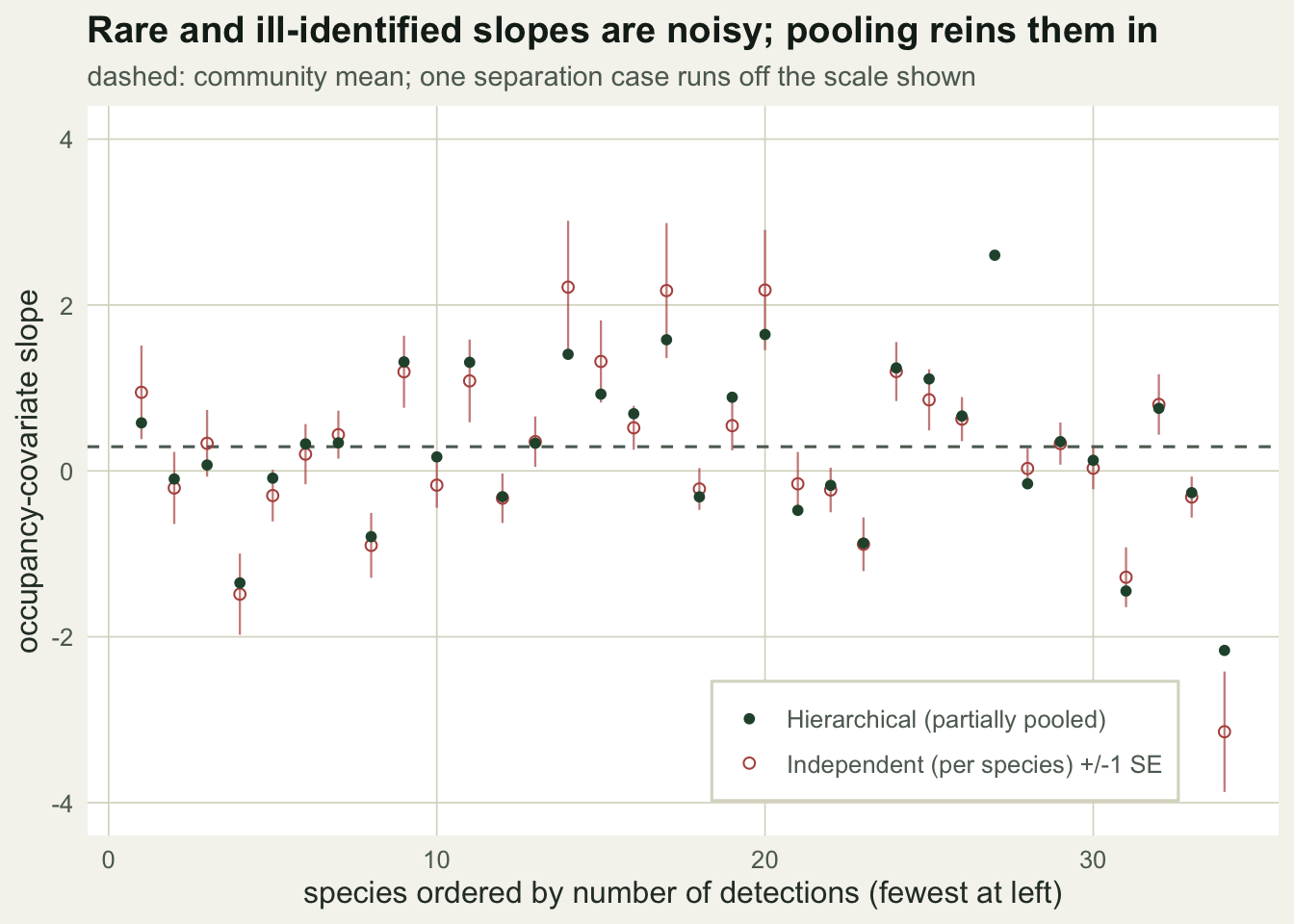
The trait relationship is what the model is really after. Plotting slope against trait puts the naive line next to the community relationship the integrated model fits, with the pooled slopes around that line.
b1h <- hp[4]; b0h <- hp[3]; xr <- range(tr)
lh <- data.frame(tr=seq(xr[1],xr[2],length=50)); lh$y <- b0h + b1h*lh$tr
ln <- data.frame(tr=lh$tr, y=coef(naive)[1] + coef(naive)[2]*lh$tr)
dpt <- data.frame(tr=tr, mle=mle[,"b"], hier=bhat)
ggplot() +
  geom_point(data=dpt, aes(tr, mle), colour=te_brick, shape=1, size=1.8) +
  geom_point(data=dpt, aes(tr, hier), colour=te_forest, size=1.8) +
  geom_line(data=ln, aes(tr, y, linetype="Naive two-stage (OLS on MLE slopes)"), colour=te_gold, linewidth=0.8) +
  geom_line(data=lh, aes(tr, y, linetype="Hierarchical community relationship"), colour=te_forest, linewidth=0.8) +
  scale_linetype_manual(NULL, values=c("Naive two-stage (OLS on MLE slopes)"="dashed","Hierarchical community relationship"="solid")) +
  coord_cartesian(ylim=c(-4,4)) +
  labs(x="species trait (standardised)", y="occupancy-covariate slope",
       title="A trait explains how species respond to the gradient",
       subtitle="hollow: independent slopes; filled: pooled") +
  theme_te() + theme(legend.position = "inside", legend.position.inside = c(0.35,0.9),
                     legend.background=element_rect(fill="#ffffff",colour=te_line))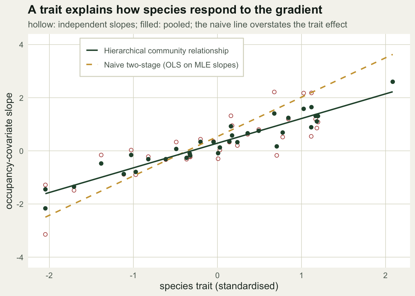
Across all species the gain is plain: the spread of the slope estimates falls from 2.07 for the independent fits to 0.98 for the pooled ones, and the mean distance from the true slopes falls from 0.543 to 0.259.
What to take away
Two-stage analyses are convenient, but regressing noisy estimates on a predictor treats every species as equally informative when some are barely informative at all. The integrated model weights each species by how much it actually tells us. The cost is the same exchangeability assumption as before: species slopes are treated as draws around a common trait line, and if a subgroup breaks that pattern the single relationship will paper over it. Whether the fitted model captures the data it was given is a question for checking a community occupancy model. The starting point, without covariates, is multi-species occupancy models.
References
- Dorazio & Royle 2005 Journal of the American Statistical Association 100(470):389-398 (10.1198/016214505000000015)
- Zipkin, DeWan & Royle 2009 Journal of Applied Ecology 46(4):815-822 (10.1111/j.1365-2664.2009.01664.x)
- Pollock, Tingley, Morris, Golding, O’Hara, Parris, Vesk & McCarthy 2014 Methods in Ecology and Evolution 5(5):397-406 (10.1111/2041-210X.12180)
- Jamil, Ozinga, Kleyer & ter Braak 2013 Journal of Vegetation Science 24(6):988-1000 (10.1111/j.1654-1103.2012.12036.x)
- Ovaskainen, Tikhonov, Norberg, Guillaume Blanchet, Duan, Dunson, Roslin & Abrego 2017 Ecology Letters 20(5):561-576 (10.1111/ele.12757)
- Kery & Royle 2016. Applied Hierarchical Modeling in Ecology, Volume 1. Academic Press. ISBN 978-0-12-801378-6