Species richness by data augmentation

Estimate how many species a survey missed. A community occupancy model with data augmentation counts the undetected tail in base R, and beats a Chao estimator.

Count the species you detected and you have a lower bound, not the richness of the community. The species you never saw are exactly the ones that are scarce or hard to detect, and they leave no direct trace in the data. A raw tally undercounts, and the shortfall grows as detection gets worse.

Data augmentation turns the community occupancy model into a richness estimator. We pad the observed species list with a large block of all-zero “potential” species, give each member of this enlarged pool an inclusion switch, and let the model decide how many of the padded species belong in the community. The number switched on, added to the species we saw, is the estimate of total richness, and it comes with a full posterior. This tutorial builds the estimator in base R and sets it against the observed count and a Chao estimator.

A survey that misses species

We simulate a community of 60 species across 70 sites with 3 visits each. Occupancy and detection vary among species on the logit scale, and the low-detectability tail means some species are never recorded.

library(ggplot2); library(dplyr)
logit <- qlogis; expit <- plogis

te_ink<-"#16241d"; te_body<-"#2c3a31"; te_forest<-"#275139"; te_faint<-"#5d6b61"
te_sage<-"#93a87f"; te_paper<-"#f5f4ee"; te_line<-"#dad9ca"; te_brick<-"#b5534e"; te_gold<-"#cda23f"
theme_te <- function(base_size=12){
  theme_minimal(base_size=base_size) +
    theme(plot.background=element_rect(fill=te_paper,colour=NA),
          panel.background=element_rect(fill="#ffffff",colour=NA),
          panel.grid.minor=element_blank(),
          panel.grid.major=element_line(colour=te_line,linewidth=0.3),
          axis.title=element_text(colour=te_body), axis.text=element_text(colour=te_faint),
          plot.title=element_text(colour=te_ink,face="bold"),
          plot.subtitle=element_text(colour=te_faint,size=rel(0.9)),
          legend.text=element_text(colour=te_faint,size=rel(0.8)))
}

set.seed(221)
Strue <- 60L; R <- 70L; K <- 3L
lpsi_t <- rnorm(Strue, logit(0.22), 1.15)         # community occupancy
lp_t   <- rnorm(Strue, logit(0.16), 1.10)         # community detection (a low tail)
psi_t  <- expit(lpsi_t); p_t <- expit(lp_t)
z_t    <- matrix(rbinom(Strue*R, 1, psi_t), Strue, R)
Yfull  <- matrix(rbinom(Strue*R, K, ifelse(z_t==1, p_t, 0)), Strue, R)

detected <- rowSums(Yfull > 0) > 0
Yobs <- Yfull[detected, , drop=FALSE]             # only species seen at least once
Sobs <- nrow(Yobs)
c(true_richness = Strue, observed = Sobs, missed = Strue - Sobs)

true_richness      observed        missed 
           60            53             7 

The survey recorded 53 of the 60 species and missed 7, a shortfall of 12 per cent. Those are real species living at the sites; they simply never showed up over three visits.

What a Chao estimator says

Incidence-based Chao2 corrects the observed count using the species seen at exactly one site (Q1) and exactly two sites (Q2): a community with many singletons probably hides more species. It is a useful lower bound but leans on those rare-frequency counts alone.

inc <- rowSums(Yobs > 0)                           # sites each observed species was seen at
Q1 <- sum(inc==1); Q2 <- sum(inc==2)
chao2   <- if (Q2>0) Sobs + Q1^2/(2*Q2) else Sobs + Q1*(Q1-1)/2
chao2bc <- Sobs + ((R-1)/R) * Q1*(Q1-1) / (2*(Q2+1))   # bias-corrected form
round(c(Q1=Q1, Q2=Q2, chao2=chao2, chao2_bc=chao2bc), 1)

      Q1       Q2    chao2 chao2_bc 
     5.0      6.0     55.1     54.4 

Here Chao2 returns 55.1 and its bias-corrected form 54.4, both short of the true 60. With only 5 singletons the estimator has little to work with, and strong detection heterogeneity is precisely the situation where it undercounts.

Augmenting the community

Add 120 all-zero species to the observed list, and give every species in this pool of size M an inclusion indicator w that is one if the species is really part of the community. Each pool member also carries an occupancy and detection probability drawn from the community distributions. A species that was detected must be in (w = 1); for an all-zero padded species, w is uncertain, and its probability of belonging depends on how easily it could have gone undetected even if present. Total richness is N = sum(w).

Maug <- 120L; M <- Sobs + Maug
Y <- rbind(Yobs, matrix(0L, Maug, R))              # padded species are all zero
ndet <- rowSums(Y>0); nzero <- R - ndet
Sy <- rowSums(Y*(Y>0)); SKy <- rowSums((K-Y)*(Y>0))
is_obs <- c(rep(TRUE, Sobs), rep(FALSE, Maug))
# marginal occupancy log-likelihood for one species (occupancy state summed out)
logLocc <- function(lpsi, lp){
  psi <- expit(lpsi); p <- expit(lp)
  ndet*log(psi) + Sy*log(p) + SKy*log(1-p) + nzero*log(psi*(1-p)^K + (1-psi))
}

The sampler draws the species probabilities and hyperparameters with Metropolis, the inclusion indicators and the inclusion rate Omega with Gibbs. A padded species only contributes its detection likelihood when it is switched on, so switched-off species are just draws from the community prior.

ni <- 16000L; nb <- 6000L; nt <- 2L
lpsi <- rep(logit(0.2), M); lp <- rep(logit(0.2), M); w <- rep(1L, M)
mps <- logit(0.2); sps <- 1; mp <- logit(0.2); sp <- 1; Omega <- 0.5
t_ls<-0.4; t_lp<-0.4; t_mu<-0.15; t_lsd<-0.15
keep <- seq(nb+1, ni, by=nt); nk <- length(keep); kk <- 0L
Nsup <- numeric(nk); HYP <- matrix(NA, nk, 4)

for (it in 1:ni){
  ll <- logLocc(lpsi, lp)
  prop <- lpsi + rnorm(M,0,t_ls)               # occupancy logits (Metropolis)
  a <- w*logLocc(prop,lp)+dnorm(prop,mps,sps,log=TRUE) - (w*ll+dnorm(lpsi,mps,sps,log=TRUE))
  au <- log(runif(M)) < a; lpsi[au] <- prop[au]; ll <- logLocc(lpsi, lp)
  prop <- lp + rnorm(M,0,t_lp)                 # detection logits (Metropolis)
  a <- w*logLocc(lpsi,prop)+dnorm(prop,mp,sp,log=TRUE) - (w*ll+dnorm(lp,mp,sp,log=TRUE))
  au <- log(runif(M)) < a; lp[au] <- prop[au]
  # inclusion indicators for padded all-zero species (Gibbs)
  ll0 <- logLocc(lpsi, lp)                     # probability of all zeros if present
  pw <- Omega*exp(ll0) / (Omega*exp(ll0) + (1-Omega))
  w <- ifelse(is_obs, 1L, rbinom(M,1,pw))
  Omega <- rbeta(1, 1+sum(w), 1+M-sum(w))      # inclusion rate (Gibbs)
  # community means and spreads (Metropolis)
  pr <- mps+rnorm(1,0,t_mu)
  if (log(runif(1)) < sum(dnorm(lpsi,pr,sps,log=TRUE))-sum(dnorm(lpsi,mps,sps,log=TRUE))) mps <- pr
  pr <- exp(log(sps)+rnorm(1,0,t_lsd))
  if (log(runif(1)) < sum(dnorm(lpsi,mps,pr,log=TRUE))+dnorm(pr,0,2.5,log=TRUE)+log(pr)-
                      sum(dnorm(lpsi,mps,sps,log=TRUE))-dnorm(sps,0,2.5,log=TRUE)-log(sps)) sps <- pr
  pr <- mp+rnorm(1,0,t_mu)
  if (log(runif(1)) < sum(dnorm(lp,pr,sp,log=TRUE))-sum(dnorm(lp,mp,sp,log=TRUE))) mp <- pr
  pr <- exp(log(sp)+rnorm(1,0,t_lsd))
  if (log(runif(1)) < sum(dnorm(lp,mp,pr,log=TRUE))+dnorm(pr,0,2.5,log=TRUE)+log(pr)-
                      sum(dnorm(lp,mp,sp,log=TRUE))-dnorm(sp,0,2.5,log=TRUE)-log(sp)) sp <- pr
  if (it>nb && ((it-nb) %% nt == 0)){ kk<-kk+1L; Nsup[kk]<-sum(w); HYP[kk,]<-c(mps,sps,mp,sp) }
}
qN <- quantile(Nsup, c(0.025,0.5,0.975))
round(c(post_mean=mean(Nsup), median=qN[2], lower=qN[1], upper=qN[3]), 1)

  post_mean  median.50%  lower.2.5% upper.97.5% 
       62.5        62.0        54.0        75.0 

Reading the estimate

The augmentation posterior puts total richness at a median of 62 with a 95 per cent interval from 54 to 75. That interval covers the true 60, sits clearly above the observed 53, and reaches past Chao2 at 55.1. The model estimates substantial detection heterogeneity, with a detection standard deviation of about 1.33 on the logit scale, which is why the undetected tail is there to be recovered in the first place.

dfN <- data.frame(N=Nsup)
ggplot(dfN, aes(N)) +
  geom_histogram(binwidth=1, fill=te_sage, colour="#ffffff", linewidth=0.15) +
  geom_vline(xintercept=Sobs, colour=te_faint, linetype="dotted", linewidth=0.7) +
  geom_vline(xintercept=chao2, colour=te_gold, linetype="dashed", linewidth=0.7) +
  geom_vline(xintercept=Strue, colour=te_brick, linewidth=0.8) +
  annotate("text", x=Sobs, y=Inf, label="observed", colour=te_faint, angle=90, vjust=-0.4, hjust=1.1, size=3) +
  annotate("text", x=chao2, y=Inf, label="Chao2", colour=te_gold, angle=90, vjust=1.2, hjust=1.1, size=3) +
  annotate("text", x=Strue, y=Inf, label="true richness", colour=te_brick, angle=90, vjust=-0.4, hjust=1.1, size=3) +
  labs(x="community richness N (species present, detected or not)", y="posterior draws",
       title="The community holds more species than were seen",
       subtitle="observed count and Chao2 sit below the truth; the posterior reaches it") +
  theme_te()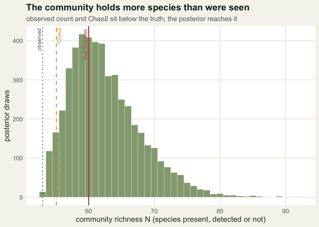

Figure 1: Posterior distribution of community richness, with the observed count, Chao2 and the true value marked.

The mechanism is clearest in the frequency of detection. Most observed species were recorded at only a handful of sites, and the model fills in a block of species at zero incidence: the ones present but never caught.

tab <- as.data.frame(table(factor(inc, levels=1:max(inc)))); names(tab) <- c("sites","species")
tab$sites <- as.integer(as.character(tab$sites))
und  <- mean(Nsup) - Sobs
zero <- data.frame(sites=0, species=und)
ggplot() +
  geom_col(data=tab, aes(sites, species), fill=te_forest, width=0.8) +
  geom_col(data=zero, aes(sites, species), fill=te_brick, width=0.8, alpha=0.55) +
  annotate("text", x=0, y=und+0.6, label="inferred\nundetected", colour=te_brick, size=3, lineheight=0.9) +
  scale_x_continuous(breaks=0:max(inc)) +
  labs(x="number of sites where a species was detected (incidence)", y="number of species",
       title="Rare species dominate, and some are never seen",
       subtitle="green: observed incidence counts; red: species inferred at zero incidence") +
  theme_te()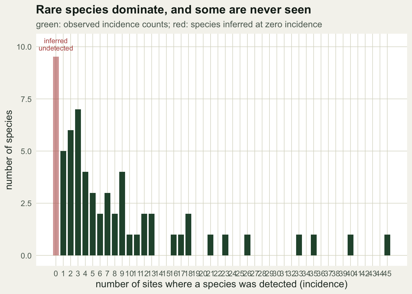

Figure 2: Number of species by how many sites they were detected at, with the inferred undetected species at zero incidence.

Cautions

The augmentation block must be large enough that the posterior for N never presses against the top of the pool; if it does, enlarge the block and refit. Richness is a genuinely uncertain quantity, so a wide interval is the honest result, not a defect, and reporting the posterior rather than a single number is the point. The estimate also rests on the community distribution and on species being exchangeable draws from it. If detection heterogeneity is even stronger or more structured than a single logit-normal allows, the tail can still be undercounted, which is why the fitted model deserves the scrutiny in checking a community occupancy model. The same augmentation trick estimates population size for a single closed population in Bayesian closed capture-recapture; here it is lifted to the level of species.

Related tutorials

• Multi-species occupancy models
• Checking a community occupancy model
• Bayesian closed capture-recapture
• N-mixture models for abundance

References

• Dorazio, Royle, Soderstrom & Glimskar 2006 Ecology 87(4):842-854 (10.1890/0012-9658(2006)87[842:ESRAAB]2.0.CO;2)
• Royle, Dorazio & Link 2007 Journal of Computational and Graphical Statistics 16(1):67-85 (10.1198/106186007X181425)
• Kery & Royle 2008 Journal of Applied Ecology 45(2):589-598 (10.1111/j.1365-2664.2007.01441.x)
• Chao 1987 Biometrics 43(4):783-791 (10.2307/2531532)
• Colwell, Chao, Gotelli, Lin, Mao, Chazdon & Longino 2012 Journal of Plant Ecology 5(1):3-21 (10.1093/jpe/rtr044)
• Iknayan, Tingley, Furnas & Beissinger 2014 Trends in Ecology and Evolution 29(2):97-106 (10.1016/j.tree.2013.10.012)
• Kery & Royle 2016. Applied Hierarchical Modeling in Ecology, Volume 1. Academic Press. ISBN 978-0-12-801378-6