library(ggplot2); library(dplyr); library(tidyr)
logit <- qlogis; expit <- plogis

te_ink<-"#16241d"; te_body<-"#2c3a31"; te_forest<-"#275139"; te_faint<-"#5d6b61"
te_sage<-"#93a87f"; te_paper<-"#f5f4ee"; te_line<-"#dad9ca"; te_brick<-"#b5534e"
theme_te <- function(base_size=12){
  theme_minimal(base_size=base_size) +
    theme(plot.background=element_rect(fill=te_paper,colour=NA),
          panel.background=element_rect(fill="#f5f4ee",colour=NA),
          panel.grid.minor=element_blank(),
          panel.grid.major=element_line(colour=te_line,linewidth=0.3),
          axis.title=element_text(colour=te_body), axis.text=element_text(colour=te_faint),
          plot.title=element_text(colour=te_ink,face="bold"),
          plot.subtitle=element_text(colour=te_faint,size=rel(0.9)),
          legend.text=element_text(colour=te_faint,size=rel(0.8)),
          strip.text=element_text(colour=te_ink,face="bold"))
}Checking a community occupancy model
ecology tutorial
R
occupancy
hierarchical models
Bayesian statistics
MCMC
model diagnostics
A community occupancy model can return sensible parameters yet fit badly. A posterior predictive check in base R catches unmodelled detection heterogeneity.
A fitted community occupancy model always returns numbers: community means, a spread among species, per-species estimates. None of that tells you whether the model actually describes the data. A model can be comfortably wrong, handing back plausible parameters while missing a feature of the assemblage entirely. The way to find out is to simulate data from the fitted model and compare it against what was observed.
A posterior predictive check does exactly that. For each draw from the posterior, generate a fresh dataset, compute a discrepancy measure on both the real and the simulated data, and see whether the observed discrepancy is unusual against the spread of replicated ones. This tutorial builds the check in base R for a community occupancy model, and uses it to catch a common failure: detection that varies among sites but is modelled as if it does not.
Two communities, one modelled feature missing
We build two datasets. Both have species-specific occupancy and detection drawn from community distributions. In the first, detection for a species is the same at every site. In the second, an unmeasured site condition raises or lowers detection everywhere at that site, so some sites are easy to survey and others hard. The model we fit assumes the first situation, so it is correct for one dataset and wrong for the other.
simdat <- function(seed, hetero=FALSE, sigma_site=1.2){
  set.seed(seed)
  S <- 35L; R <- 90L; K <- 4L
  lpsi <- rnorm(S, logit(0.40), 1.0); lp <- rnorm(S, logit(0.35), 0.7)
  psi <- expit(lpsi); z <- matrix(rbinom(S*R,1,psi), S, R)
  if (hetero){ u <- rnorm(R, 0, sigma_site)                  # site survey-condition effect
    P <- expit(outer(lp, rep(1,R)) + matrix(u, S, R, byrow=TRUE))
  } else { P <- matrix(expit(lp), S, R) }                    # detection constant across sites
  y <- matrix(rbinom(S*R, K, ifelse(z==1, P, 0)), S, R)
  list(y=y, S=S, R=R, K=K)
}
dat_h <- simdat(606,  hetero=FALSE)   # detection homogeneous across sites
dat_g <- simdat(4602, hetero=TRUE)    # detection varies by site (unmodelled)
The model, the discrepancy, and the check
The fitted model is the community occupancy model with a species detection probability that does not depend on site. The discrepancy measure is a Freeman-Tukey statistic on the number of detections per site, summed over species and visits: it compares each site total against what the model expects, on a square-root scale that stabilises the variance. If detection really varies among sites, the observed site totals spread out more than the model can produce, and the statistic picks that up.
The routine samples the model with Metropolis-within-Gibbs and, at each kept draw, computes the discrepancy for the observed data and for one simulated replicate. The Bayesian p-value is the fraction of draws where the replicate discrepancy is at least as large as the observed one; a value near one-half means the observed data look like the model’s own output, while a value near zero means they do not. The ratio of mean observed to mean replicated discrepancy is a companion lack-of-fit measure that should sit near one for a good fit.
fit_ppc <- function(dat, ni=14000L, nb=5000L, nt=2L){
  y<-dat$y; S<-dat$S; R<-dat$R; K<-dat$K
  ndet<-rowSums(y>0); nzero<-R-ndet; Sy<-rowSums(y*(y>0)); SKy<-rowSums((K-y)*(y>0))
  LL <- function(lpsi,lp){ psi<-expit(lpsi); p<-expit(lp)                    # occupancy state summed out
    ndet*log(psi) + Sy*log(p) + SKy*log(1-p) + nzero*log(psi*(1-p)^K + (1-psi)) }
  lpsi<-logit(pmin(pmax((ndet+.5)/(R+1),.02),.98)); lp<-rep(logit(.35),S)
  mps<-0; sps<-1; mp<-logit(.35); sp<-1
  t_ls<-.3; t_lp<-.26; t_mu<-.14; t_lsd<-.14
  keep<-seq(nb+1,ni,by=nt); nk<-length(keep); kk<-0L
  Dobs<-colSums(y)                                                           # observed detections per site
  Tobs<-Trep<-numeric(nk); ge<-logical(nk); DREP<-matrix(NA,nk,R)
  for (it in 1:ni){
    ll<-LL(lpsi,lp)
    pr<-lpsi+rnorm(S,0,t_ls); a<-LL(pr,lp)+dnorm(pr,mps,sps,log=TRUE)-(ll+dnorm(lpsi,mps,sps,log=TRUE)); au<-log(runif(S))<a; lpsi[au]<-pr[au]; ll<-LL(lpsi,lp)
    pr<-lp+rnorm(S,0,t_lp);   a<-LL(lpsi,pr)+dnorm(pr,mp,sp,log=TRUE)-(ll+dnorm(lp,mp,sp,log=TRUE));   au<-log(runif(S))<a; lp[au]<-pr[au]
    pr<-mps+rnorm(1,0,t_mu); if(log(runif(1))<sum(dnorm(lpsi,pr,sps,log=TRUE))-sum(dnorm(lpsi,mps,sps,log=TRUE)))mps<-pr
    pr<-exp(log(sps)+rnorm(1,0,t_lsd)); if(log(runif(1))<sum(dnorm(lpsi,mps,pr,log=TRUE))+dnorm(pr,0,2.5,log=TRUE)+log(pr)-sum(dnorm(lpsi,mps,sps,log=TRUE))-dnorm(sps,0,2.5,log=TRUE)-log(sps))sps<-pr
    pr<-mp+rnorm(1,0,t_mu);  if(log(runif(1))<sum(dnorm(lp,pr,sp,log=TRUE))-sum(dnorm(lp,mp,sp,log=TRUE)))mp<-pr
    pr<-exp(log(sp)+rnorm(1,0,t_lsd));  if(log(runif(1))<sum(dnorm(lp,mp,pr,log=TRUE))+dnorm(pr,0,2.5,log=TRUE)+log(pr)-sum(dnorm(lp,mp,sp,log=TRUE))-dnorm(sp,0,2.5,log=TRUE)-log(sp))sp<-pr
    if (it>nb && ((it-nb)%%nt==0)){ kk<-kk+1L
      psi<-expit(lpsi); p<-expit(lp); ED<-sum(psi*K*p)                       # expected detections per site
      Tobs[kk]<-sum((sqrt(Dobs)-sqrt(ED))^2)                                 # Freeman-Tukey, observed
      zr<-matrix(rbinom(S*R,1,psi),S,R); yr<-matrix(rbinom(S*R,K,ifelse(zr==1,p,0)),S,R)
      Drep<-colSums(yr); Trep[kk]<-sum((sqrt(Drep)-sqrt(ED))^2); ge[kk]<-Trep[kk]>=Tobs[kk]; DREP[kk,]<-Drep
    }
  }
  list(bp=mean(ge), chat=mean(Tobs)/mean(Trep), Tobs=Tobs, Trep=Trep, Dobs=Dobs, DREP=DREP)
}
rh <- fit_ppc(dat_h)   # homogeneous data
rg <- fit_ppc(dat_g)   # heterogeneous data
round(c(bp_homogeneous=rh$bp, chat_homogeneous=rh$chat,
        bp_heterogeneous=rg$bp, chat_heterogeneous=rg$chat), 3)
bp_homogeneous chat_homogeneous bp_heterogeneous chat_heterogeneous
0.564 0.967 0.000 6.566 For the homogeneous dataset the Bayesian p-value is 0.564 and the lack-of-fit ratio is 0.97, both pointing to a good fit: the observed data are unremarkable against the model’s own replicates. For the heterogeneous dataset the p-value collapses to 0 and the ratio climbs to 6.57: the observed discrepancy is far larger than anything the model produces. Bayesian p-values are often called conservative, pulled toward one-half, but the pull belongs to the discrepancy rather than to the method. A statistic the model can absorb by refitting its own parameters degenerates toward one-half and detects nothing at all; one the model cannot absorb keeps enough power to matter. The variance-based discrepancy used here is the well-behaved case, so a value this close to zero is a strong signal rather than a borderline one. The parameter estimates in the second case look perfectly reasonable, which is the whole point. Nothing in the fitted community means or spreads announces the problem; only the check does.
mk <- function(r,lab) data.frame(To=r$Tobs, Tr=r$Trep, scen=lab)
d1 <- rbind(mk(rh, sprintf("homogeneous detection  (p = %.2f)", rh$bp)),
            mk(rg, sprintf("unmodelled site heterogeneity  (p = %.2f)", rg$bp)))
ggplot(d1, aes(To, Tr)) +
  geom_abline(slope=1, intercept=0, colour=te_faint, linewidth=0.5) +
  geom_point(colour=te_forest, alpha=0.25, size=0.8) +
  geom_blank(aes(x=Tr, y=To)) +  # each panel spans both ranges, so the identity line is drawn in both
  facet_wrap(~scen, scales="free") +
  labs(x="discrepancy for observed data  T(y)", y="discrepancy for replicated data  T(y_rep)",
       title="A posterior predictive check separates fit from misfit",
       subtitle="points below the identity line: the model under-predicts the observed discrepancy") +
  theme_te()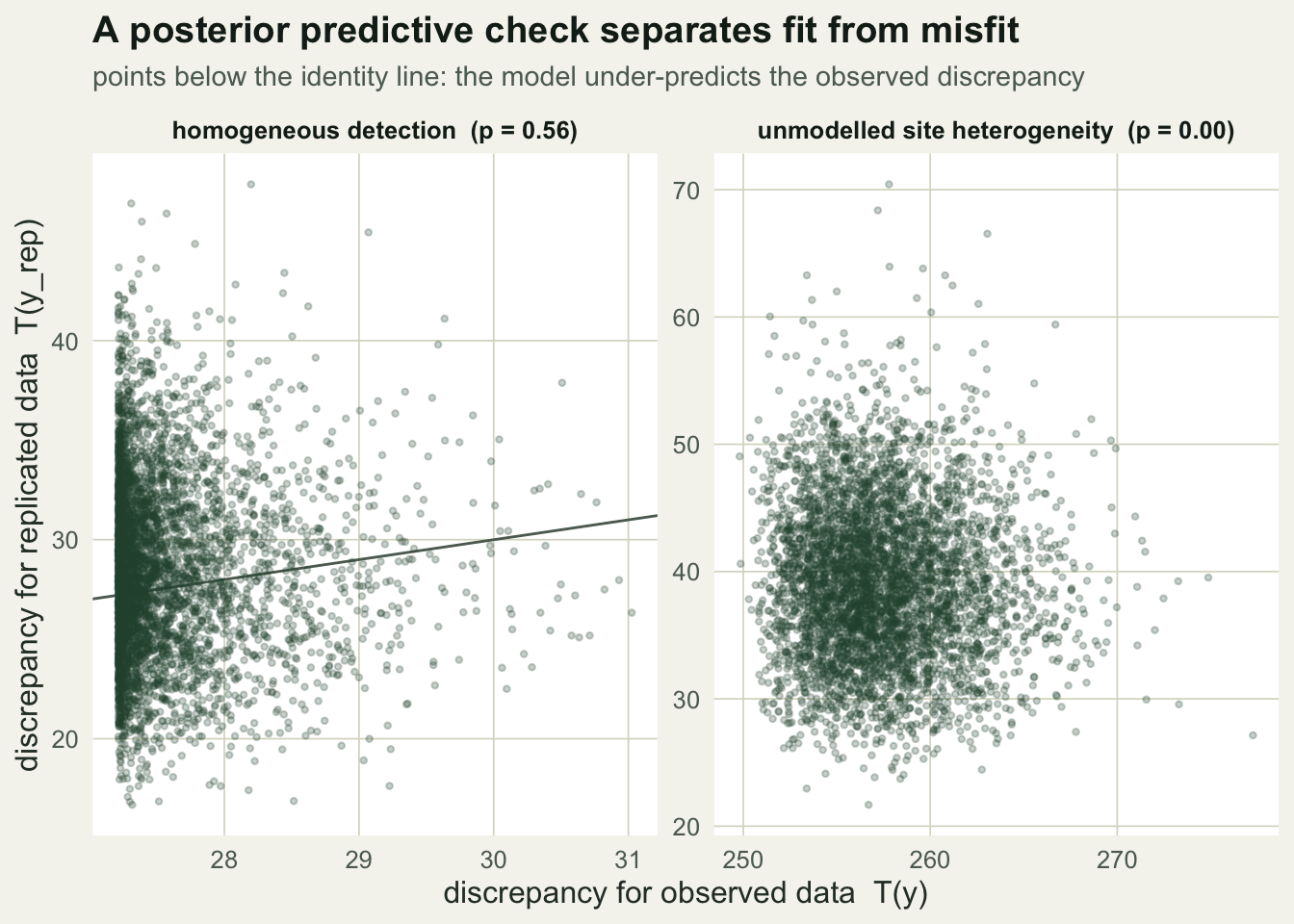
Where the misfit lives
The check flags a problem; the next question is what kind. Plotting the observed distribution of detections per site against the model’s posterior-predictive distribution shows it directly. For the homogeneous data the two match. For the heterogeneous data the observed spread is far wider than the model expects, because easy sites pile up detections and hard sites yield almost none, and a single site-constant detection probability cannot make data that dispersed.
den <- function(r,lab) rbind(
  data.frame(v=r$Dobs,             src="observed",              scen=lab),
  data.frame(v=as.numeric(r$DREP), src="posterior-predictive", scen=lab))
d2 <- rbind(den(rh,"homogeneous detection"), den(rg,"unmodelled site heterogeneity"))
ggplot(d2, aes(v)) +
  geom_density(data=subset(d2,src=="posterior-predictive"), aes(colour="posterior-predictive"),
               fill=te_sage, alpha=0.25, linewidth=0.5) +
  geom_density(data=subset(d2,src=="observed"), aes(colour="observed"), fill=NA, linewidth=0.9) +
  scale_colour_manual(NULL, values=c("observed"=te_brick,"posterior-predictive"=te_forest)) +
  facet_wrap(~scen, scales="free") +
  labs(x="detections per site (summed over species and visits)", y="density",
       title="The misfit is over-dispersion across sites",
       subtitle="observed spread far exceeds what the constant-detection model predicts") +
  theme_te() + theme(legend.position="top")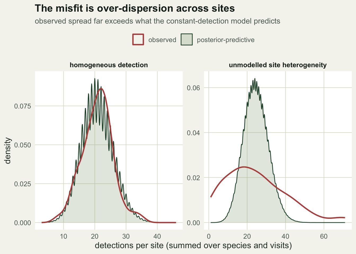
The observed per-site detections vary far more under heterogeneity, with a variance-to-mean ratio of 10.4 against 1.16 for the homogeneous data. That over-dispersion is the fingerprint the check is responding to.
The remedy, and the habit
Once the check points at among-site variation in detection, the fix follows: let detection depend on the site. If a survey condition was recorded, add it as a detection covariate; if not, add a site-level random effect on detection so the model can absorb the extra spread. Refit, and the same check should settle back toward a p-value near one-half.
The broader habit matters more than this one repair. Community models are easy to fit and easy to over-trust, and a plausible-looking set of estimates is not evidence of fit. A posterior predictive check with a discrepancy aimed at the feature you care about, whether per-site detection spread, the distribution of species detection frequencies, or observed richness, is cheap to run and hard to fool. Build it into the workflow alongside multi-species occupancy models, species richness estimation, and community covariates and traits.
References
- Gelman, Meng & Stern 1996 Statistica Sinica 6(4):733-807
- Kery & Royle 2016. Applied Hierarchical Modeling in Ecology, Volume 1. Academic Press. ISBN 978-0-12-801378-6
- Broms, Hooten & Fitzpatrick 2016 Ecology 97(7):1759-1770 (10.1890/15-1471.1)
- MacKenzie & Bailey 2004 Journal of Agricultural, Biological, and Environmental Statistics 9(3):300-318 (10.1198/108571104X3361)
- Warton, Stoklosa, Guillera-Arroita, MacKenzie & Welsh 2017 Methods in Ecology and Evolution 8(4):408-419 (10.1111/2041-210X.12761)
- Conn, Johnson, Williams, Melin & Hooten 2018 Ecological Monographs 88(4):526-542 (10.1002/ecm.1314)