library(ggplot2)

te_paper  <- "#f5f4ee"
te_ink    <- "#16241d"
te_body   <- "#2c3a31"
te_forest <- "#275139"
te_rust   <- "#b5534e"
te_gold   <- "#c9b458"
te_line   <- "#dad9ca"

theme_datasheet <- function() {
  theme_minimal(base_size = 12) +
    theme(plot.background  = element_rect(fill = te_paper, colour = NA),
          panel.background = element_rect(fill = te_paper, colour = NA),
          panel.grid.major = element_line(colour = te_line, linewidth = 0.3),
          panel.grid.minor = element_blank(),
          text             = element_text(colour = te_body),
          axis.text        = element_text(colour = te_body),
          strip.text       = element_text(colour = te_ink, face = "bold"))
}What a p-value tells you, and what it does not
R
statistics
hypothesis testing
simulation
ecology tutorial
What a p-value means, checked by simulating the null in R, and why p = 0.03 in a grazing experiment is no promise that an exact repeat will be significant.
Twelve fenced plots and twelve grazed plots on an upland pasture, and after one season the height of the tallest rowan seedling in each plot. The fenced plots grew taller seedlings on average, and t.test() returns p = 0.03. The question that follows is almost always the same: does that mean the effect is real, and would I find it again if I ran the experiment a second time?
Many posts on this site report p-values, usually in passing. This post explains what one is, on that single grazing experiment. It computes the p-value twice, once with t.test() and once by counting simulated experiments, then measures what happens when the same experiment is repeated with the same true effect and new plots. The answer to the second question turns out to be much less reassuring than p = 0.03 sounds.
The short answer. A p-value is the probability, calculated on the assumption that there is no effect at all, of getting a test statistic at least as extreme as the one you observed. It is not the probability that the effect is real, and one minus p is not the chance that a repeat would be significant. That chance is the power of the design at the true effect, which depends on the true effect and the sample size, and your p-value cannot tell you the true effect. Power worked out from the effect you happened to observe is a different number, a function of p alone. Report the estimate and its confidence interval next to the p-value, because the interval shows the uncertainty that a single p-value hides.
All data here are simulated, and every seed is in the code.
One experiment, one p-value
The simulated pasture has a real grazing effect: seedlings in fenced plots are 3.5 cm taller on average, and plots vary around their treatment mean with a standard deviation of 4 cm. These values, with twelve plots per treatment, were fixed before anything was run, chosen so that the design detects the effect about half the time. Your own experiment is one draw from a process like this, and in the question it came out between 0.01 and 0.05, so the chunk below draws experiments until one does and keeps that one.
n_plots     <- 12     # plots per treatment
sd_height   <- 4      # cm, plot-to-plot standard deviation
true_diff   <- 3.5    # cm, fenced minus grazed: the true effect in the simulation
grazed_mean <- 20     # cm

set.seed(1015)
repeat {
  grazed <- rnorm(n_plots, grazed_mean, sd_height)
  fenced <- rnorm(n_plots, grazed_mean + true_diff, sd_height)
  p_try  <- t.test(fenced, grazed)$p.value
  if (p_try > 0.01 && p_try < 0.05) break
}
test_obs <- t.test(fenced, grazed)
test_obs
    Welch Two Sample t-test

data:  fenced and grazed
t = 2.1875, df = 21.416, p-value = 0.03993
alternative hypothesis: true difference in means is not equal to 0
95 percent confidence interval:
 0.2301139 8.8936858
sample estimates:
mean of x mean of y
 23.66038  19.09848
The fenced plots are 4.56 cm taller on average, the t statistic is 2.19 and the p-value is 0.040, inside the window of the question if not exactly 0.03; nothing below depends on that difference. The header of the output says “Welch Two Sample t-test”: by default t.test() has var.equal = FALSE, so it does not assume the two groups share one variance. Pretesting variances before a t test explains why that default is the safer one to keep.
What the p-value counts
The definition has two parts that matter. The probability is computed assuming there is no effect, and it covers results “at least as extreme” as yours, not results exactly like yours. Both parts can be checked by brute force. Build a world in which grazing does nothing: both groups come from the same distribution. Run the experiment in that world a hundred thousand times, compute the t statistic each time, and count how often it is at least as far from zero as the observed 2.19:
n_null <- 1e5
pooled_sd <- sqrt((var(fenced) + var(grazed)) / 2)

set.seed(2015)
null_runs <- replicate(n_null, {
  a <- rnorm(n_plots, grazed_mean, pooled_sd)    # fenced plots, no effect
  b <- rnorm(n_plots, grazed_mean, pooled_sd)    # grazed plots
  tt <- t.test(a, b)
  c(t = unname(tt$statistic), p = tt$p.value)
})
p_counted <- mean(abs(null_runs["t", ]) >= abs(t_obs))
mc_se_p   <- sqrt(p_counted * (1 - p_counted) / n_null)
round(c(t_test = p_obs, counted = p_counted, mc_se = mc_se_p), 4)
t_test counted mc_se
0.0399 0.0386 0.0006 In 3.86 per cent of the no-effect experiments the statistic was at least as extreme as ours, against 3.99 per cent from t.test(). That is the definition at work: the p-value is a share of experiments in a world without an effect. The mean and standard deviation of that world do not matter, because the t statistic does not change when all heights are shifted or rescaled; what matters is that the two groups are identical. t.test() reads the share from a t distribution instead of counting, and Probability distributions in R: d, p, q and r explains the p functions such as pnorm(); pt(), which t.test() uses, is the same for the t distribution.
The two numbers differ by 0.13 percentage points, 2.2 Monte Carlo standard errors (one standard error, the typical size of the simulation noise, is 0.06 points here). Most of that is simulation noise, and a small part has a reason. With the same number of plots in both groups, the Welch statistic is exactly the ordinary pooled t statistic, and when both groups share one variance, as in the simulated world, its exact distribution is the t distribution with 22 degrees of freedom. The Welch test uses 21.4 here, a little fewer, so its p-value is a little larger than the exact 3.96 per cent. The counted share is 1.7 standard errors from that exact value.
The same hundred thousand null experiments show the property that everything else rests on. An exact p-value is spread evenly between zero and one when there is no effect, so p < 0.05 happens one time in twenty. Read from the exact t distribution, 4.91 per cent of the null experiments give p below 0.05 (Monte Carlo standard error 0.07); with the Welch p-values the share is 4.80 per cent, slightly lower for the reason just given. Checking a multiple-testing analysis shows the flat histogram this produces and what it looks like when it goes wrong.
Would a repeat find it again?
Now the second half of the question. Take the same pasture, the same true effect of 3.5 cm, the same twelve plots per treatment, and run the experiment many times. Each run is paired with an exact replicate: same design, same truth, new plots.
n_rep <- 30000
one_run <- function() {
  t.test(rnorm(n_plots, grazed_mean + true_diff, sd_height),
         rnorm(n_plots, grazed_mean, sd_height))$p.value
}
set.seed(3015)
p_original  <- replicate(n_rep, one_run())
p_replicate <- replicate(n_rep, one_run())

power_sim <- mean(p_original < 0.05)
power_se  <- sqrt(power_sim * (1 - power_sim) / n_rep)
round(c(power = power_sim, mc_se = power_se,
        quantile(p_original, c(0.10, 0.50, 0.90))), 4)
power mc_se 10% 50% 90%
0.5324 0.0029 0.0016 0.0420 0.3917 At the true effect of 3.5 cm this design has power 0.532 (Monte Carlo standard error 0.003): a run of the experiment gives p < 0.05 about half the time. (power.t.test(), which uses the pooled rather than the Welch test, gives 0.536.) Across runs of the same experiment the p-value moves over a very wide range. The middle run has p = 0.042; one run in ten has p below 0.0016, and one in ten has p above 0.39. Nothing changed between those runs except which plots were drawn. Cumming (2008) shows how wide this spread is across replications, and Halsey and colleagues (2015) make the same point for experimental biology.
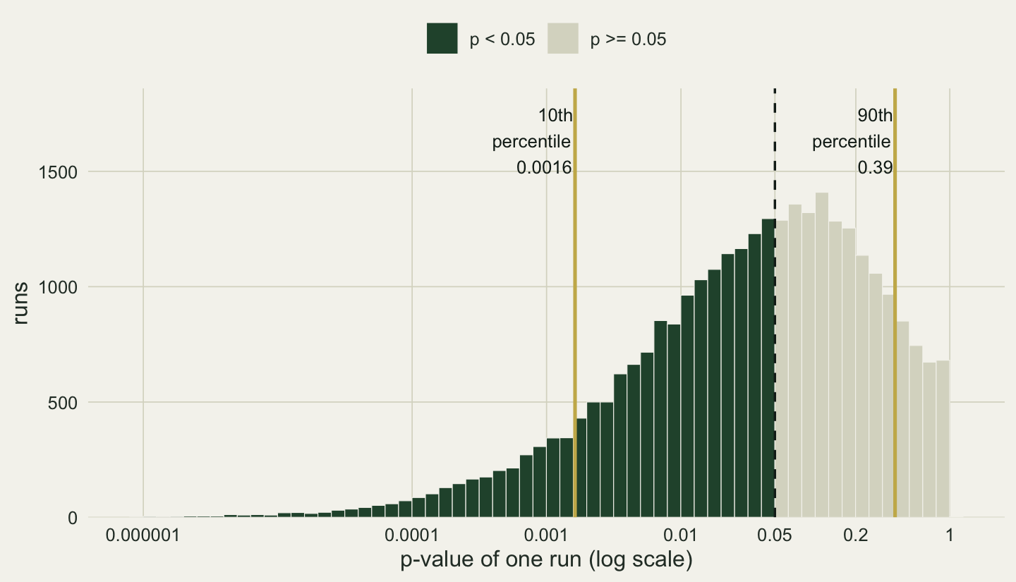
That spread already answers the question, but the question is conditional: my experiment gave p between 0.01 and 0.05, so what are the chances for the repeat? Keep only the original runs that landed in that window, as yours did, and look at their replicates:
in_window <- p_original > 0.01 & p_original < 0.05
rep_share <- mean(p_replicate[in_window] < 0.05)
rep_se    <- sqrt(rep_share * (1 - rep_share) / sum(in_window))
round(c(runs_in_window = sum(in_window), replicate_significant = rep_share,
        mc_se = rep_se, power = power_sim), 4)
runs_in_window replicate_significant mc_se
7889.0000 0.5350 0.0056
power
0.5324 # the same share after other original results
by_original <- cut(p_original, c(0, 0.001, 0.01, 0.05, 0.2, 1))
round(tapply(p_replicate < 0.05, by_original, mean), 3) (0,0.001] (0.001,0.01] (0.01,0.05] (0.05,0.2] (0.2,1]
0.552 0.540 0.535 0.527 0.525 Of the 7889 original runs with p between 0.01 and 0.05, 0.535 had a significant replicate (Monte Carlo standard error 0.006), next to the power at the true effect of 0.532. The second table shows that the share hardly depends on the original p: whether the original run gave p below 0.001 or above 0.2, the share of significant replicates stays between 0.525 and 0.552, and every group is within 1.8 Monte Carlo standard errors of the power (counting the error of both shares). This is not a coincidence of the simulation. The replicate uses new plots, so it is independent of the original run once the true effect is fixed, and its chance of p < 0.05 is the power of the design at the true effect, whatever the original p was. The simulation only confirms it.
So the honest answer to “would I find it again?” is: with the probability given by the power at the true effect, which the p-value of your experiment does not tell you. Here it is close to a coin flip, while the reading “p = 0.040, so a repeat is almost certain” would put it near one minus p, 0.96.
A published calculation is often quoted at this point, and it answers a different question. Goodman (1992) assumed that the true effect equals the one you observed, used a z-test, and found that a result at exactly p = 0.05 is followed by a significant replicate half of the time: pnorm(qnorm(0.975) - qnorm(0.975)) is 0.5. At p = 0.03 the same formula gives 0.58, and at our p of 0.040 it gives 0.54. Even that optimistic assumption leaves the chance far from one minus p. But Goodman’s number is the power at the observed effect, which is what Observed power tells you nothing calls observed power: a function of p alone. The simulated share is the power at the true effect, which p does not reveal. Apply Goodman’s formula to every original run and compare it with what the replicates did:
# Goodman's replication probability for each original run: the power at its observed effect
goodman_run <- pnorm(qnorm(1 - p_original / 2) - qnorm(0.975))
round(rbind(goodman    = tapply(goodman_run, by_original, mean),
            replicates = tapply(p_replicate < 0.05, by_original, mean)), 3)
(0,0.001] (0.001,0.01] (0.01,0.05] (0.05,0.2] (0.2,1]
goodman 0.949 0.817 0.617 0.377 0.136
replicates 0.552 0.540 0.535 0.527 0.525After an original p below 0.001, Goodman’s formula averages 0.95, but only 0.552 of those replicates reached significance; in the window of the question it averages 0.62 against a measured 0.535, and after p above 0.2 it averages 0.14 against 0.525. Goodman’s number follows the original p; the replicates follow the power at the true effect. The two land close together for our experiment only because its p is near 0.05 and the power at the true effect happens to be near one half.
What a p-value is not
Three misreadings follow from the definition; the last two have fuller treatments elsewhere on this site, so here each gets one paragraph.
A p-value is not the probability that there is no effect. It is the probability of data at least this extreme if there is no effect: a statement about the data, not about the hypothesis. p = 0.040 does not mean a 4 per cent chance that grazing does nothing; the second principle of the American Statistical Association statement on p-values (Wasserstein and Lazar 2016) says this in one line. How far apart the two probabilities are depends on how often the effects you test for are real; the section after this one prices that for this design.
A p-value is not the size of the effect. A tiny difference measured on thousands of plots gives a tiny p-value, and in a small study the runs that reach significance overestimate the effect; Power analysis by simulation in R measures that exaggeration.
A p-value above 0.05 is not evidence that there is no effect. In this design 47 per cent of runs miss a real 3.5 cm difference. Observed power tells you nothing explains why a power figure computed afterwards cannot repair that, and Testing for no effect: equivalence tests in R gives the test that can support “no effect worth caring about”.
How often is there no effect behind it?
The first misreading can be turned into a number, but only with one ingredient that no experiment supplies: how often the effects you test for are real. Picture many experiments like this one on many pastures. In a share of them, call it the prior, fencing really adds 3.5 cm; in the rest grazing does nothing. Among the experiments that end with p between 0.01 and 0.05, as yours did, what share had no effect behind them? The post already holds both kinds of run: the hundred thousand no-effect experiments of the null simulation and the 30000 runs at the true effect.
window_null <- mean(null_runs["p", ] > 0.01 & null_runs["p", ] < 0.05)   # no effect, p in the window
window_true <- mean(p_original > 0.01 & p_original < 0.05)               # true effect, p in the window
# among results of one kind, the share that came from a true null
false_share <- function(prior, from_null, from_true) {
  (1 - prior) * from_null / ((1 - prior) * from_null + prior * from_true)
}
priors <- c(0.10, 0.25, 0.50)
fpr_table <- rbind(window   = false_share(priors, window_null, window_true),
                   below_05 = false_share(priors, null_below, power_sim))
colnames(fpr_table) <- sprintf("prior %.2f", priors)
round(fpr_table, 3)
prior 0.10 prior 0.25 prior 0.50
window 0.569 0.306 0.128
below_05 0.448 0.213 0.083If one tested effect in ten of this kind is real, 57 per cent of the results in the window come from experiments in which grazing did nothing, and 45 per cent of all results with p < 0.05 do (Monte Carlo standard errors 0.5 and 0.4 points). At one in four the shares are 31 and 21 per cent, at even odds 13 and 8 per cent. The window share falls to five per cent only at a prior of 0.74. The window is worse than p < 0.05 because it leaves out the very small p-values, which the real effect often produces and a null rarely does: a run at the true effect is 6.8 times as likely as a null run to land in the window, but 11.1 times as likely to land below 0.05.
None of this needs the simulation. An exact p-value is uniform under the null, so a null run lands in the window with probability 0.04 and below 0.05 with probability 0.05. At the true effect the pooled t statistic follows a noncentral t distribution with 22 degrees of freedom and noncentrality 2.14, and the chance that it falls in the matching band is 0.259 for the window and 0.536 for p < 0.05, the power that power.t.test(strict = TRUE) returns. The simulated curves in the figure reproduce these closed forms and sit a little below them, partly because the Welch test is slightly conservative and partly by chance: 3.86 per cent of the null runs landed in the window instead of 4, and the same runs read from the exact t distribution give 3.93 per cent. With the Welch share in the formula, the six simulated values in the table are within 1.7 Monte Carlo standard errors of the closed form. The window also pools p-values near 0.01 with p-values near 0.05. In the same closed form, a p-value right at 0.040 is only 4.5 times as likely at the true effect as with no effect, against 6.5 for the window as a whole, so for a result exactly like yours the share from true nulls is higher: 67, 40 and 18 per cent at the three priors.
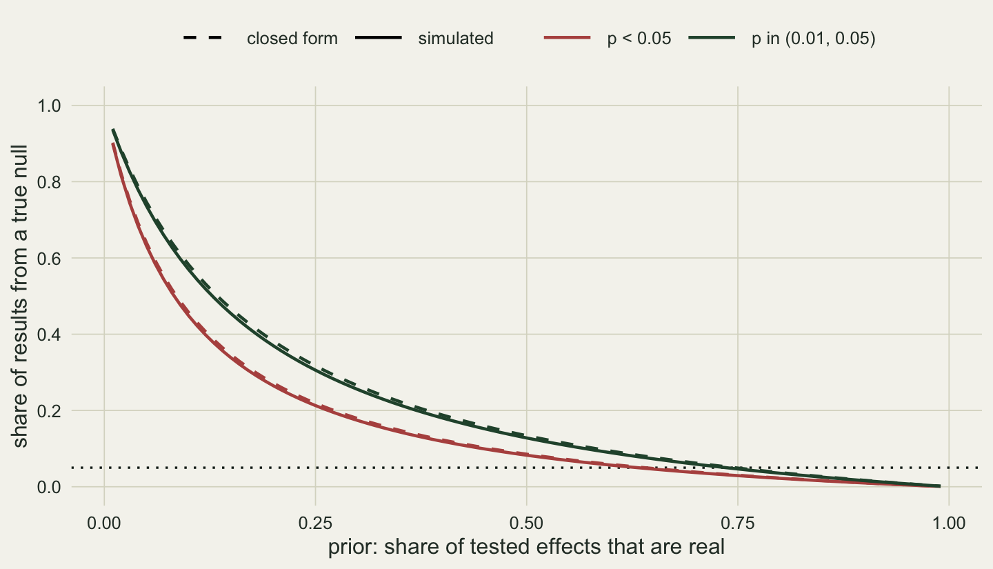
This share is not the false discovery rate of The false discovery rate and Benjamini-Hochberg, which is the expected share of false rejections among many tests and is held down by a correction; it is the same kind of ratio for one uncorrected test, with the prior supplied from outside. In a screen of many tests the prior is one minus the proportion of true nulls, which Checking a multiple-testing analysis estimates from the p-value histogram. A single experiment has no histogram, so the prior stays a judgement and the answer stays a curve. Colquhoun (2014), who calls this share the false discovery rate, works out the same share for other priors and powers, both for p below 0.05 and for p close to it.
Report the interval next to it
The fix for the grazing experiment is one line that is already in the t.test() output: the estimate with its 95 per cent confidence interval. Standard errors and confidence intervals in R explains how the interval is built and what its coverage means.
round(c(estimate = diff_obs, lower = ci_obs[1], upper = ci_obs[2]), 2)estimate lower upper
4.56 0.23 8.89 The same experiment that gave p = 0.040 says the fenced plots are between 0.23 and 8.89 cm taller. The low end is a difference nobody would notice in the field, and the high end is 1.9 times the estimate itself. The low end sits near zero because p sits near 0.05: the interval and the p-value come from the same t statistic, but the interval states the result in centimetres, where you can judge which effects are still in play. The figure repeats the experiment twenty times with the same truth.
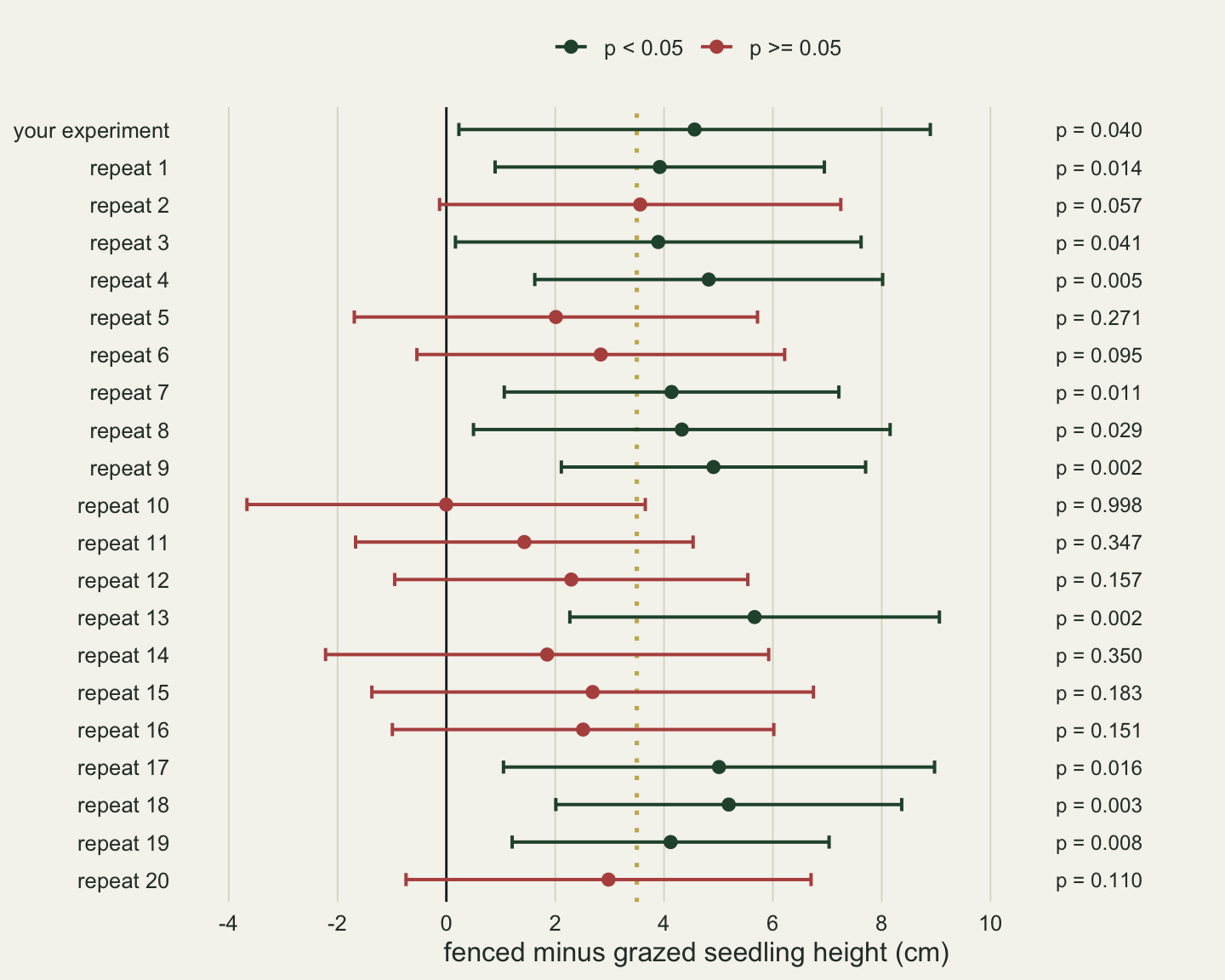
In these twenty repeats 10 gave p < 0.05, and the p-values ran from 0.0016 to 0.998. All 20 intervals of the same runs contain the true 3.5 cm, whether or not their run crossed 0.05, and each states in centimetres which effects that run leaves in play. Cumming (2008) works this contrast out in general: an interval says more about where the next result will land than the p-value does.
What to check in your own data
Before you write “significant”, read what t.test() or summary() actually ran. For t.test() the header names the test, and the default is Welch; for lm() and glm() each coefficient’s p-value tests that one coefficient against zero with the others in the model.
Put the estimate and its confidence interval in the sentence, not only the p-value: “fenced plots were 4.6 cm taller (95 per cent CI 0.2 to 8.9)” says more than “p = 0.040”, and a reader can see at once whether small effects are still in play.
When you plan a follow-up or judge whether a result should replicate, ask what the power of the design is. At the true effect, that power is the chance a repeat reaches significance, not one minus p. Because the true effect is unknown, compute the power for the smallest effect you care about: it tells you whether a repeat could reliably detect an effect of that size. Do not plug in the effect you observed; that gives observed power, Goodman’s number, which only restates p.
If a result sits just below 0.05, treat it as what the spread of p-values above shows it to be: a single draw from a wide range. Do not sort results into real and not real at the threshold; Comparing significance is not a test shows what goes wrong when two results on either side of 0.05 are read as different.
Honest limits
The whole post uses one design: normal plot heights, equal spread in both groups, twelve plots each, and one true effect chosen so that the power sits near one half. With a stronger effect or more plots the power at the true effect, and so the replication share, rises; the point is that the share is set by that power and not by the p-value, nor by the power computed at the observed effect. The replication share was measured with the true effect fixed. In a real literature true effects vary and some are zero, and then the share of significant replicates after p between 0.01 and 0.05 depends on that mixture, which no single experiment reveals. How often is there no effect behind it? prices one consequence of that mixture in its simplest form, a fixed share of true nulls with every real effect exactly 3.5 cm: the share of window results that have no effect behind them, drawn as a curve because the mixture is unknown. The example experiment was chosen from the simulation because its p-value fell in the window of the question; the interval figures in the last section describe that one draw and twenty repeats, not a coverage study, which Standard errors and confidence intervals in R runs properly.
References
Colquhoun D 2014 Royal Society Open Science 1(3):140216 (10.1098/rsos.140216)
Cumming G 2008 Perspectives on Psychological Science 3(4):286-300 (10.1111/j.1745-6924.2008.00079.x)
Goodman SN 1992 Statistics in Medicine 11(7):875-879 (10.1002/sim.4780110705)
Halsey LG, Curran-Everett D, Vowler SL, Drummond GB 2015 Nature Methods 12(3):179-185 (10.1038/nmeth.3288)
Wasserstein RL, Lazar NA 2016 The American Statistician 70(2):129-133 (10.1080/00031305.2016.1154108)