library(ggplot2)

te_paper  <- "#f5f4ee"
te_ink    <- "#16241d"
te_body   <- "#2c3a31"
te_forest <- "#275139"
te_rust   <- "#b5534e"
te_gold   <- "#c9b458"
te_line   <- "#dad9ca"

theme_datasheet <- function() {
  theme_minimal(base_size = 12) +
    theme(plot.background  = element_rect(fill = te_paper, colour = NA),
          panel.background = element_rect(fill = te_paper, colour = NA),
          panel.grid.major = element_line(colour = te_line, linewidth = 0.3),
          panel.grid.minor = element_blank(),
          text             = element_text(colour = te_body),
          axis.text        = element_text(colour = te_body),
          strip.text       = element_text(colour = te_ink, face = "bold"))
}Probability distributions in R: d, p, q and r
R
statistics
count data
simulation
ecology tutorial
The d, p, q and r functions in R on ecological counts and lengths, why 1 - ppois(k) is not the chance of at least k, and checking parameters by simulation.
A field protocol for a rare orchid says: revisit in June every quadrat that held at least three seedlings in April. The planning team knows from earlier years that seedlings are scattered at random at about 2.5 per quadrat, and wants to know how many of the 120 quadrats will need a second visit. Someone types 1 - ppois(3, 2.5) into R, gets an answer, and books the field days. The answer is wrong by almost half, and nothing in R says so.
R handles every probability distribution with four functions that share a stem and differ in their first letter: dpois(), ppois(), qpois() and rpois() for the Poisson, and the same four letters in front of binom, norm, nbinom, gamma, lnorm and the rest. Much of the code on this site uses them, usually without comment. This post explains what each letter returns, measures a trap that is easy to fall into with counts, and then checks three places where R’s parameters are not the ones a textbook or another program may have taught you.
The short answer. d gives the probability of exactly one value (for a count) or the height of the density curve (for a measurement). p gives the probability of a value at or below a cut-off. q runs p backwards: you give a probability and get the value. r draws random values. For “at least k” on a count, use ppois(k - 1, lambda, lower.tail = FALSE), never 1 - ppois(k, lambda). And before trusting a distribution you have not used before, draw a large sample with its r function and compare the sample mean and variance with what you expect.
All data here are simulated or come straight from the distributions; every seed is in the code.
Four letters, one stem
Take the orchid seedlings first. If they fall at random with a mean of 2.5 per quadrat, the count in one quadrat follows a Poisson distribution with lambda = 2.5. dpois() gives the probability of each exact count:
lambda <- 2.5                       # mean seedlings per quadrat
round(dpois(0:7, lambda), 4)
[1] 0.0821 0.2052 0.2565 0.2138 0.1336 0.0668 0.0278 0.0099sum(dpois(0:100, lambda)) # all the probabilities add up to one[1] 1An empty quadrat has probability 0.082, a quadrat with exactly two seedlings 0.257. ppois() adds these up from zero to a cut-off, so it answers “at most”:
ppois(2, lambda) # P(X <= 2)[1] 0.5438131sum(dpois(0:2, lambda)) # the same sum, written out[1] 0.5438131stopifnot(isTRUE(all.equal(ppois(2, lambda), sum(dpois(0:2, lambda)))))The chance that a quadrat holds at most two seedlings is 0.544. The “at most”, with the cut-off included, is the whole story of the trap in the next section.
The same letters work for any distribution. A newt that is present at a pond is detected on a single visit with probability 0.3, and the pond is visited five times. The number of visits with a detection is binomial, and dbinom(0, ...) is the chance of missing the newt on every visit:
visits <- 5
p_det  <- 0.3
dbinom(0, size = visits, prob = p_det)     # never detected in five visits
[1] 0.16807set.seed(1014)
sim_det <- rbinom(1e5, size = visits, prob = p_det)
mean(sim_det == 0) # share of simulated ponds with no detection[1] 0.16804An occupied pond is missed with probability 0.168, and in a hundred thousand simulated ponds 0.168 had no detection (the Monte Carlo standard error of that share, the typical size of the simulation noise, is 0.0012). This is the r letter’s everyday job: produce data from a known model so that you can check a formula, a model fit or a sampling design against it. Power analysis by simulation in R builds a whole study design this way, and A reproducible statistical workflow in R explains where to put set.seed() so the draws come out the same every time.
For a measurement such as body length, d means something different. Here are adult newts with a mean total length of 0.10 m and a standard deviation of 0.008 m:
dnorm(0.10, mean = 0.10, sd = 0.008) # length in metres[1] 49.86779dnorm(100, mean = 100, sd = 8) # the same newts in millimetres[1] 0.04986779pnorm(0.11, 0.10, 0.008) - pnorm(0.09, 0.10, 0.008) # P(0.09 m < length < 0.11 m)[1] 0.7887005pnorm(110, 100, 8) - pnorm(90, 100, 8) # the same interval in millimetres[1] 0.7887005The first line returns 49.9, which cannot be a probability. For a continuous variable dnorm() returns a density: probability per unit of the measurement, here per metre. A newt length is spread over a few centimetres, so the density per metre is large. Measured in millimetres the same newts give a density of 0.0499, a thousand times smaller, while the probability of a length between 9 and 11 cm is 0.789 in both units. Probabilities for a measurement always come from pnorm() differences, areas under the curve; the probability of any single exact length is zero. qnorm() and its relative qt() turn up whenever a confidence interval is built, which Standard errors and confidence intervals in R covers.
At least k: the trap with counts
Back to the orchid protocol. The team wants P(X >= 3), the chance a quadrat holds three or more seedlings. The habit many people bring from the normal distribution is “the upper tail is one minus p”, and it gives:
k <- 3
wrong <- 1 - ppois(k, lambda)                          # P(X > 3), i.e. at least 4
right <- ppois(k - 1, lambda, lower.tail = FALSE)      # P(X > 2), i.e. at least 3
c(wrong = wrong, right = right)
wrong right
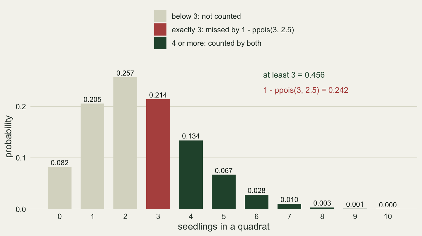
0.2424239 0.4561869 ppois(k, lambda) includes k itself, so one minus it is the chance of MORE than k: at least four seedlings, not at least three. The R help page for the Poisson says it in one line: with lower.tail = TRUE (the default) the probabilities are P(X <= x), otherwise P(X > x). To get “at least k” you ask for “more than k - 1”. The next chunk checks both statements and the size of the gap:
stopifnot(
  isTRUE(all.equal(ppois(k, lambda), sum(dpois(0:k, lambda)))),                    # default: P(X <= k)
  isTRUE(all.equal(ppois(k, lambda, lower.tail = FALSE), 1 - ppois(k, lambda))),   # FALSE: P(X > k)
  isTRUE(all.equal(right, 1 - ppois(k - 1, lambda))),
  isTRUE(all.equal(right - wrong, dpois(k, lambda)))                               # the missing bar
)
# relative error of the one-minus version for "at least 6"
rel6 <- 100 * (1 - (1 - ppois(6, lambda)) / ppois(5, lambda, lower.tail = FALSE))
stopifnot(rel6 > 100 * (1 - wrong / right))

set.seed(3014)
seedlings <- rpois(1e6, lambda)
sim_at_least <- mean(seedlings >= k)
sim_more     <- mean(seedlings > k)
mcse <- sqrt(sim_at_least * (1 - sim_at_least) / length(seedlings))
round(c(simulated_at_least = sim_at_least, simulated_more_than = sim_more, mc_se = mcse), 4)
simulated_at_least simulated_more_than mc_se
0.4560 0.2423 0.0005 The correct chance is 0.456; the one-minus version gives 0.242, 47 per cent too low. A million simulated quadrats settle which is which: 0.456 of them hold at least three seedlings (Monte Carlo standard error 0.0005), and 0.242 hold more than three. The gap between the two answers is exactly the probability of k itself, dpois(3, 2.5) = 0.214: the wrong formula leaves out the bar at three. A Poisson distribution peaks near its mean, so the missing bar, the absolute error, is largest when the threshold is close to the mean count, as it is here. In relative terms the error grows further out: for at least 6 seedlings the one-minus version is 66 per cent too low.
For the protocol, the expected number of revisits is the number of quadrats times the probability:
n_quadrats <- 120
round(c(booked_with_wrong = n_quadrats * wrong, needed = n_quadrats * right), 1)
booked_with_wrong needed
29.1 54.7 The team would plan for 29 revisits and meet about 55. The same slip appears in every “at least” with a discrete count: a detection rule, a minimum group size, a threshold number of nests. With the newt data, “call a pond occupied if the newt is detected on at least two of five visits” needs pbinom(1, 5, 0.3, lower.tail = FALSE):
occ_wrong <- 1 - pbinom(2, visits, p_det)
occ_right <- pbinom(1, visits, p_det, lower.tail = FALSE)
c(wrong = occ_wrong, right = occ_right)
wrong right
0.16308 0.47178 stopifnot(isTRUE(all.equal(occ_right - occ_wrong, dbinom(2, visits, p_det))),
# the negative binomial follows the same rule
isTRUE(all.equal(pnbinom(2, size = 2, mu = 3, lower.tail = FALSE),
1 - sum(dnbinom(0:2, size = 2, mu = 3)))))An occupied pond passes the rule with probability 0.472; the one-minus version says 0.163, the chance of at least three detections.
For a normal or any other continuous distribution the slip does no harm, because a single value has probability zero and “more than” equals “at least”. That is how the habit forms. With counts it matters every time.
lower.tail = FALSE has a second use. For a far tail, 1 - ppois() subtracts a number that is almost one from one, and floating-point arithmetic loses the answer:
c(one_minus = 1 - ppois(30, lambda), lower_tail = ppois(30, lambda, lower.tail = FALSE)) one_minus lower_tail
0.00000e+00 2.34756e-23 stopifnot(1 - ppois(30, lambda) == 0, ppois(30, lambda, lower.tail = FALSE) > 0)The one-minus form returns exactly zero, while lower.tail = FALSE returns \(2.35 \times 10^{-23}\). A zero probability inside a likelihood becomes minus infinity on the log scale, so for tail probabilities the argument is the safer habit anyway.
Quantiles of a count jump in steps
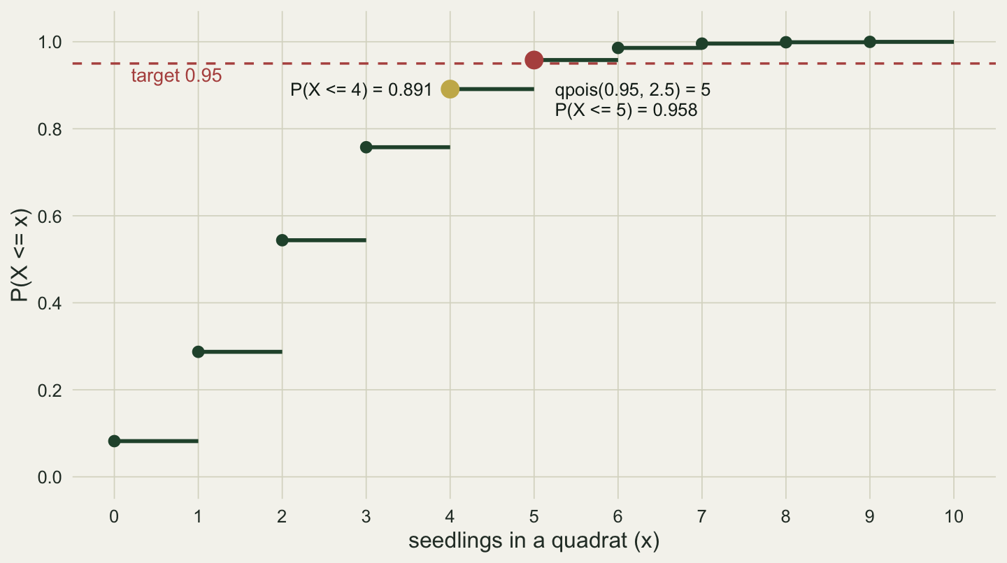
qpois() runs the other way: give it a probability, get back a count. The help page defines it as the smallest integer x with P(X <= x) >= p. For a count that is not the same as “the value with 95 per cent below it”:
q95 <- qpois(0.95, lambda)
round(c(q95 = q95, P_at_most_q95 = ppois(q95, lambda), P_at_most_one_less = ppois(q95 - 1, lambda)), 4)
q95 P_at_most_q95 P_at_most_one_less
5.0000 0.9580 0.8912 stopifnot(ppois(q95, lambda) >= 0.95, ppois(q95 - 1, lambda) < 0.95,
# a central 90 per cent interval from qpois() covers at least 0.90
ppois(q95, lambda) - ppois(qpois(0.05, lambda) - 1, lambda) >= 0.90)The 95th percentile of seedlings per quadrat is 5, but P(X <= 5) is 0.958, not 0.95; one seedling lower, P(X <= 4) is only 0.891. No count sits at exactly 0.95, because the cumulative probability jumps from one step to the next, and qpois() returns the first step that reaches the target. An interval built from qpois() or qnbinom() quantiles, as in the prediction band of Poisson and negative binomial GLMs in R, therefore covers at least its nominal share of the fitted distribution, and often more (estimation error in the fitted mean is a separate matter). If the exact coverage matters, report ppois() at the returned value next to it.
Parameters that differ from the textbook
The functions agree on their letters; they do not all agree with other software on their parameters (Bolker 2008, chapter 4, sets out these parameterisations for ecologists). Three cases catch ecologists often enough to check by simulation, each with a hundred thousand draws.
Negative binomial. rnbinom() takes either size and prob or size and mu. In the prob form the help page describes the number of failures before size successes, with mean size (1 - prob) / prob; prob is not the probability of anything you counted in the field. The mu form, the one ecologists use for aggregated counts, sets the mean directly, and the variance is mu + mu^2 / size, so size is the aggregation parameter k (small size, strong clumping; how badly k is estimated from few samples is the subject of Negative binomial k from small host samples). The two forms describe the same distribution when prob = size / (size + mu):
nb_size <- 2; nb_mu <- 3
nb_prob <- nb_size / (nb_size + nb_mu)
set.seed(2014)
draws_prob <- rnbinom(1e5, size = nb_size, prob = nb_prob)
draws_mu   <- rnbinom(1e5, size = nb_size, mu = nb_mu)
nb_check <- rbind(
  stated_prob_form = c(mean = nb_size * (1 - nb_prob) / nb_prob, var = nb_size * (1 - nb_prob) / nb_prob^2),
  simulated_prob   = c(mean(draws_prob), var(draws_prob)),
  stated_mu_form   = c(nb_mu, nb_mu + nb_mu^2 / nb_size),
  simulated_mu     = c(mean(draws_mu), var(draws_mu)))
round(nb_check, 3)
mean var
stated_prob_form 3.000 7.500
simulated_prob 3.005 7.465
stated_mu_form 3.000 7.500
simulated_mu 3.001 7.491stopifnot(isTRUE(all.equal(nb_check["stated_prob_form", ], nb_check["stated_mu_form", ], check.attributes = FALSE)),
isTRUE(all.equal(dnbinom(0:20, size = nb_size, prob = nb_prob),
dnbinom(0:20, size = nb_size, mu = nb_mu))))With size = 2, prob = 0.4 in one form and mu = 3 in the other, both help-page formulas give a mean of 3.0 and a variance of 7.5. The prob draws average 3.005 with variance 7.47, and the mu draws 3.001 with variance 7.49. Some texts and programs count successes instead of failures, or write the variance as a linear rather than quadratic function of the mean (Linden and Mantyniemi 2011 give a negative binomial with two overdispersion parameters that covers these different mean-variance relationships for ecological counts), so a k or a p copied from elsewhere may mean something else in R.
Gamma. rgamma() has a rate and a scale, one the inverse of the other, and the third position in the argument list belongs to rate. Code written as rgamma(n, 2, 0.5) by someone who thinks in shape and scale gets a rate of 0.5, which is a scale of 2:
stopifnot(identical(names(formals(rgamma))[1:4], c("n", "shape", "rate", "scale")))
set.seed(4014)
g_positional <- rgamma(1e5, 2, 0.5)                   # read by R as shape = 2, rate = 0.5
g_scale      <- rgamma(1e5, shape = 2, scale = 0.5)   # what a shape-scale reader meant
gamma_check <- rbind(
  positional = c(stated_mean = 2 / 0.5, mean = mean(g_positional), stated_var = 2 / 0.5^2, var = var(g_positional)),
  scale_0.5  = c(2 * 0.5, mean(g_scale), 2 * 0.5^2, var(g_scale)))
round(gamma_check, 3)
stated_mean mean stated_var var
positional 4 4.004 8.0 8.035
scale_0.5 1 1.002 0.5 0.498The mean is shape times scale, so the positional call averages 4.00 and the named scale = 0.5 call 1.00: a fourfold difference from one unnamed argument. Naming every parameter (shape =, rate = or scale =) removes the question.
Lognormal. rlnorm(n, meanlog, sdlog) takes the mean and standard deviation of the LOG of the variable. exp(meanlog) is the median, not the mean; the mean is exp(meanlog + sdlog^2 / 2):
set.seed(5014)
ml <- log(10); sl <- 0.8
lengths_ln <- rlnorm(1e5, meanlog = ml, sdlog = sl)
round(c(exp_meanlog = exp(ml), sim_median = median(lengths_ln),
        stated_mean = exp(ml + sl^2 / 2), sim_mean = mean(lengths_ln)), 3)
exp_meanlog sim_median stated_mean sim_mean
10.000 9.947 13.771 13.698 With meanlog = log(10) and sdlog = 0.8, the draws have a median of 9.95 and a mean of 13.70 against a stated mean of 13.77. What this does to predictions from a model fitted on the log scale is the subject of Back-transforming a log-scale model.
The check in all three cases is the same few lines: draw a hundred thousand values, and compare mean() and var() (or the median and mean, for the lognormal) with the formula on the help page. It takes a second and it settles what the parameters mean in the version of R you are running.
What to check in your own data
Every time you write “at least” with a count, look for a - 1 or a lower.tail = FALSE with k - 1. If you find 1 - ppois(k, ...), 1 - pbinom(k, ...) or 1 - pnbinom(k, ...), you are computing “more than k”.
When a threshold rule, a detection rule or a power calculation rests on a tail probability, check it against a simulation with the matching r function: mean(rpois(1e6, lambda) >= k) takes a moment and catches the off-by-one immediately.
When you report a quantile or an interval for a count, add the actual probability at the returned value with the p function, since it will not be exactly the nominal one.
Name the parameters of every r, d, p and q call for distributions with more than one parameterisation (size, prob, mu, shape, rate, scale), and when you take a parameter value from a paper or another program, find out which form it used before you plug it in.
Honest limits
The trap is measured for the Poisson and the binomial, and the lower-tail rule is checked once for the negative binomial; the other discrete distributions in R document the same P(X <= x) convention, but the post does not test each of them. The post covers six families and three parameterisation traps and leaves out many others (the Weibull, the beta, the truncated and zero-inflated forms that need extra packages). The simulation checks confirm means, variances and one median, not the full shape of a distribution. And a correct probability is only as good as the model under it: real seedlings are rarely scattered as a Poisson process, and if they are clumped the at-least-three share is different again.
References
Bolker BM 2008 Ecological Models and Data in R, chapter 4 (ISBN 978-0-691-12522-0)
Linden A, Mantyniemi S 2011 Ecology 92(7):1414-1421 (10.1890/10-1831.1)
R Core Team 2024 R documentation: The Poisson distribution (https://stat.ethz.ch/R-manual/R-devel/library/stats/html/Poisson.html)
R Core Team 2024 R documentation: The negative binomial distribution (https://stat.ethz.ch/R-manual/R-devel/library/stats/html/NegBinomial.html)
R Core Team 2024 R documentation: The gamma distribution (https://stat.ethz.ch/R-manual/R-devel/library/stats/html/GammaDist.html)