library(ggplot2)
library(patchwork)

te_paper  <- "#f5f4ee"
te_ink    <- "#16241d"
te_body   <- "#2c3a31"
te_forest <- "#275139"
te_rust   <- "#b5534e"
te_gold   <- "#c9b458"
te_line   <- "#dad9ca"

theme_datasheet <- function() {
  theme_minimal(base_size = 12) +
    theme(plot.background  = element_rect(fill = te_paper, colour = NA),
          panel.background = element_rect(fill = te_paper, colour = NA),
          panel.grid.major = element_line(colour = te_line, linewidth = 0.3),
          panel.grid.minor = element_blank(),
          text             = element_text(colour = te_body),
          plot.title       = element_text(colour = te_ink, face = "bold"),
          plot.subtitle    = element_text(colour = te_body),
          axis.text        = element_text(colour = te_body),
          strip.text       = element_text(colour = te_ink, face = "bold"))
}Negative binomial k from small host samples
R
parasitology
count data
simulation
ecology tutorial
From 15 to 40 hosts the aggregation k often has no finite estimate. Measuring in R how the rule for those samples creates false k-burden relationships.
Twenty lakes, twenty five perch from each, every eye opened under a dissecting microscope and every fluke metacercaria counted. The mean burden runs from well under one fluke per fish in the clear upland lakes to a few dozen in the shallow eutrophic ones where the snail hosts are thick. Each lake gets a mean and a negative binomial aggregation parameter \(k\), and the obvious next question is comparative: does aggregation change with burden, as a plot of \(k\) against mean burden seems to say? It is the question that reviews of wildlife parasite data ask across many host samples at once; Shaw and Dobson (1995) related mean burden to variance and to negative binomial parameters over published datasets from many host and parasite taxa. This post does not test whether any published pattern of that kind is an artefact, and the reporting rules below push the slope in opposite directions.
That plot is where this post starts, because \(k\) from twenty five hosts is a noisy thing, and at low burdens it is often not a number at all. The maximum likelihood estimate of \(k\) exists only when the variance computed with divisor \(n\) exceeds the sample mean. When it does not, the likelihood keeps rising as \(k\) grows and the software returns a huge value, a warning, or nothing, and the analyst has to write down something. Whatever is written down then enters the comparison.
The small sample behaviour of the \(k\) estimators is old and known. Pieters and colleagues (1977) compared estimators of the negative binomial parameters in small samples; Gregory and Woolhouse (1993) showed by simulation that the level of aggregation is systematically underestimated as fewer hosts are sampled, and warned that sample sizes unequal among host age classes can produce artefactual age-aggregation curves; Lloyd-Smith (2007) showed that the maximum likelihood estimate is biased upward in small samples of highly overdispersed data, that intervals built from its asymptotic variance cover less often than nominal, and in his simulations set samples with the variance below the mean to an infinite \(k\). So what follows is a demonstration, not a discovery: that \(k\) estimated from few hosts can manufacture a pattern across groups is close to the Gregory and Woolhouse warning, although here every lake has the same number of hosts and only the mean burden differs. Its applied angle is the reporting rule for the samples with no finite estimate, and what that rule does to a comparison across host groups whose true \(k\) is identical.
Three posts here sit next to it. Parasite burdens truncated by host death fits \(k\) to two hundred and forty hosts and attacks it through missing heavy burdens; the sample is large and fixed, and the question is truncation. Sequential sampling for pest decisions feeds a wrong \(k\) into a sampling plan and measures the damage, but never estimates \(k\). Dispersion checks when the counts are small calibrates the yes or no question of overdispersion at small counts, not the size of \(k\). Here the samples are complete, the model is right, and only the number of hosts, the mean burden and the reporting rule move.
When the likelihood has no top
For a fixed \(k\) the maximum likelihood estimate of the negative binomial mean is the sample mean, whatever \(k\) is, so the likelihood for \(k\) can be profiled with the mean held at \(\bar x\) and nothing else to fit. That profile is one curve in one variable.
k_min <- 1e-4; k_max <- 1e6         # search limits for k
chi_cut <- qchisq(0.95, 1) / 2      # drop in log likelihood for a 95 per cent profile interval

ll_tab <- function(ux, wt, kk, m) sum(wt * dnbinom(ux, size = kk, mu = m, log = TRUE))

fit_k <- function(x) {
  m <- mean(x)
  if (m == 0) return(c(ml = NA, lo = NA, hi = NA, mom = NA, m = 0))
  tb <- table(x); ux <- as.numeric(names(tb)); wt <- as.vector(tb)
  v_n <- mean((x - m)^2)                         # variance with divisor n
  s2 <- var(x)                                   # variance with divisor n - 1
  mom <- if (s2 > m) m^2 / (s2 - m) else Inf     # moment estimate
  ll_pois <- sum(wt * dpois(ux, m, log = TRUE))  # the limit as k grows
  if (v_n <= m) {
    ml <- Inf; ll_max <- ll_pois
  } else {
    opt <- optimize(function(lk) -ll_tab(ux, wt, exp(lk), m),
                    c(log(k_min), log(k_max)), tol = 1e-5)
    ml <- exp(opt$minimum); ll_max <- -opt$objective
  }
  prof <- function(lk) ll_tab(ux, wt, exp(lk), m) - (ll_max - chi_cut)
  lo <- exp(uniroot(prof, c(log(k_min), if (is.finite(ml)) log(ml) else log(k_max)),
                    tol = 1e-4)$root)
  hi <- if (!is.finite(ml) || ll_pois >= ll_max - chi_cut) Inf else
    exp(uniroot(prof, c(log(ml), log(k_max)), tol = 1e-4)$root)
  c(ml = ml, lo = lo, hi = hi, mom = mom, m = m)
}
The rule in fit_k is the whole of the non-finite problem. If the variance computed with divisor \(n\) is at or below the mean, the estimate is set to infinity without searching; otherwise the likelihood is maximised over \(\log k\). The profile interval is every \(k\) whose log likelihood lies within 1.92 of the maximum, and its upper end is open whenever the Poisson limit itself is inside that band. That the variance rule and the search agree is a claim, so it is checked before anything relies on it.
n_chk <- 4000
set.seed(4101)
rule_tab <- t(replicate(n_chk, {
  x <- rnbinom(15, size = 1, mu = 0.8)
  m <- mean(x)
  if (m == 0) return(c(NA, NA, NA))
  tb <- table(x); ux <- as.numeric(names(tb)); wt <- as.vector(tb)
  opt <- optimize(function(lk) -ll_tab(ux, wt, exp(lk), m), c(log(k_min), log(k_max)))
  c(rule = mean((x - m)^2) > m, search = opt$minimum < log(k_max) - 1,
    split = mean((x - m)^2) <= m & var(x) > m)
}))
rule_tab <- rule_tab[!is.na(rule_tab[, 1]), ]
n_rule <- nrow(rule_tab)
n_disagree <- sum(rule_tab[, 1] != rule_tab[, 2])
share_nonfin_chk <- mean(rule_tab[, 1] == 0)
share_split <- mean(rule_tab[, 3])
Across 4000 samples of fifteen hosts with a mean of 0.8 and a true \(k\) of 1, the variance rule and a search over \(\log k\) up to a million disagree in 0 samples, and 21.6 per cent of the samples have no finite estimate. The divisor matters at the margin: in 4.8 per cent of the samples the usual variance with divisor \(n - 1\) exceeds the mean, so the moment estimate is finite, while the maximum likelihood estimate is not.
set.seed(4102)
lake_draws <- replicate(40, rnbinom(25, size = 0.5, mu = 0.6), simplify = FALSE)
lake_fits <- t(sapply(lake_draws, fit_k))
i_fin <- which(is.finite(lake_fits[, "ml"]) & is.finite(lake_fits[, "hi"]))[1]
i_inf <- which(!is.finite(lake_fits[, "ml"]))[1]
ex_fin <- lake_fits[i_fin, ]; ex_inf <- lake_fits[i_inf, ]
var_n <- function(x) mean((x - mean(x))^2)
ex_v_fin <- var_n(lake_draws[[i_fin]]); ex_v_inf <- var_n(lake_draws[[i_inf]])
ex_zero_inf <- sum(lake_draws[[i_inf]] == 0)
prof_curve <- function(x, lab) {
  m <- mean(x); lk <- seq(log(0.01), log(1e4), length.out = 300)
  ll <- vapply(lk, function(v) sum(dnbinom(x, size = exp(v), mu = m, log = TRUE)), 0)
  data.frame(k = exp(lk), rel = ll - max(ll), sample = lab)
}
prof_df <- rbind(prof_curve(lake_draws[[i_fin]], "variance above the mean"),
                 prof_curve(lake_draws[[i_inf]], "variance at or below the mean"))
Two lakes drawn from the same population make the point, both with twenty five fish, a mean of 0.6 flukes and a true \(k\) of 0.5. In the first the sample mean is 0.36 and the variance 0.79; the likelihood has a peak at \(k\) = 0.14 and the profile interval runs from 0.03 to 0.94. In the second the mean is 0.20, the variance 0.16, and 20 of the twenty five fish carry no flukes. The likelihood rises all the way to the Poisson, there is no peak to report, and the only thing the data say is that \(k\) is at least 0.20.
ggplot(prof_df, aes(k, rel, colour = sample)) +
  geom_hline(yintercept = -chi_cut, colour = te_body, linetype = "dashed", linewidth = 0.5) +
  geom_vline(xintercept = 0.5, colour = te_body, linetype = "dotted", linewidth = 0.5) +
  geom_line(linewidth = 1) +
  scale_x_log10(breaks = c(0.01, 0.1, 1, 10, 100, 1000, 10000),
                labels = c("0.01", "0.1", "1", "10", "100", "1000", "10000")) +
  scale_colour_manual(values = c(te_forest, te_rust), name = NULL) +
  coord_cartesian(ylim = c(-8, 0.2)) +
  labs(x = "aggregation parameter k (log scale)", y = "log likelihood minus its maximum",
       title = "One peak, and one likelihood with no top",
       subtitle = "dashed line: 95 per cent profile cut, dotted line: true k") +
  theme_datasheet() + theme(legend.position = "bottom")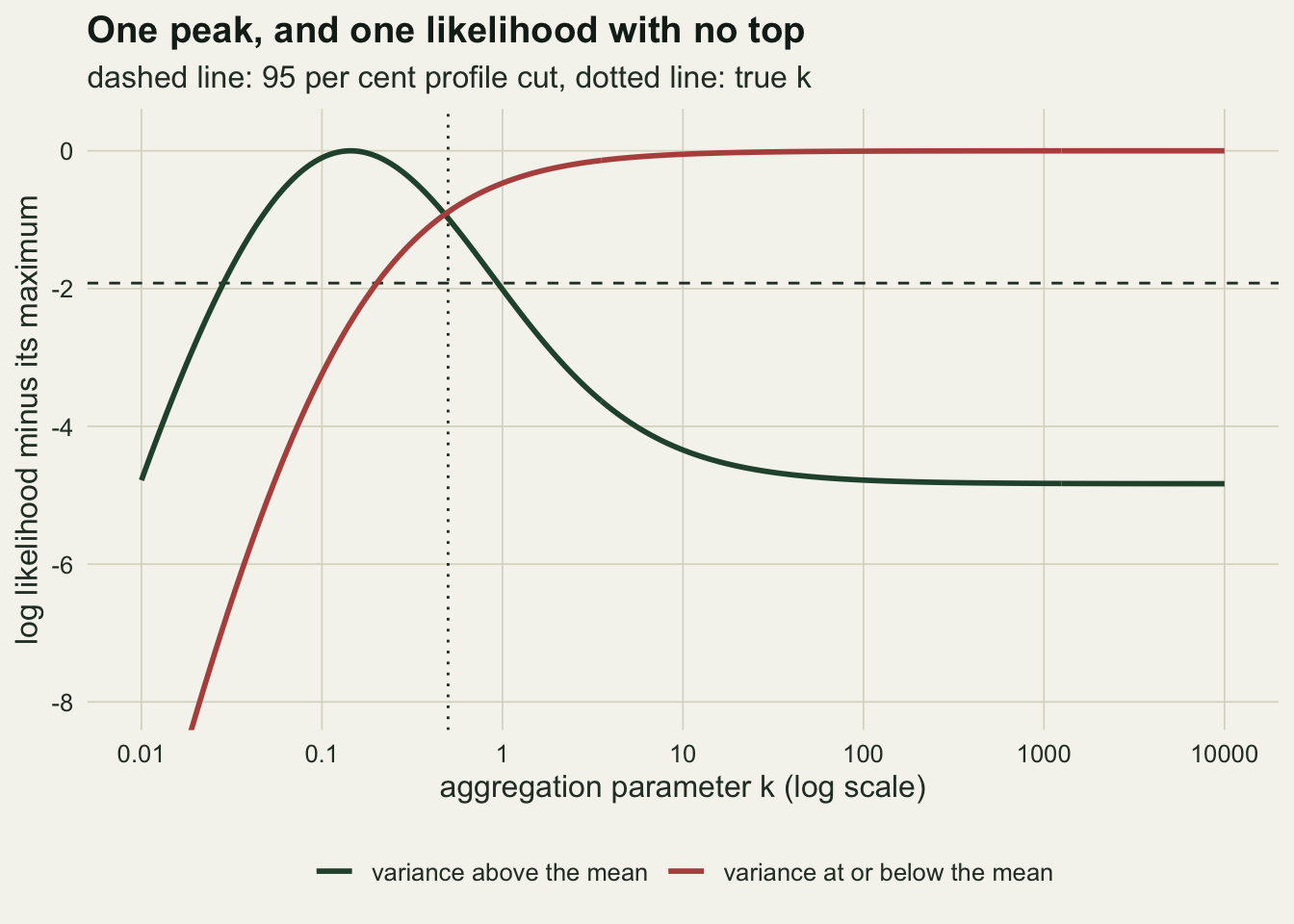
The non-finite share over hosts, burden and k
The design grid crosses five host sample sizes, five mean burdens and four true values of \(k\), fixed before any cell was run. Each of the hundred cells gets the same number of simulated samples.
n_set <- c(15, 25, 40, 80, 150)
mu_set <- c(0.5, 1, 3, 10, 30)
k_set <- c(0.2, 0.5, 1, 2)
n_rep_grid <- 500

grid_cell <- function(n, mu, k) {
  fits <- t(vapply(seq_len(n_rep_grid), function(i) fit_k(rnbinom(n, size = k, mu = mu)),
                   numeric(5)))
  ok <- !is.na(fits[, "ml"]); fits <- fits[ok, , drop = FALSE]
  fin <- is.finite(fits[, "ml"]); fin_mom <- is.finite(fits[, "mom"])
  covers <- fits[, "lo"] <= k & fits[, "hi"] >= k
  c(n = n, mu = mu, k = k, all_zero = mean(!ok), nonfin = mean(!fin),
    ml_med = median(fits[fin, "ml"]) / k, mom_med = median(fits[fin_mom, "mom"]) / k,
    over2 = mean(fits[, "ml"] > 2 * k), under_half = mean(fits[, "ml"] < k / 2),
    cover = mean(covers), open_hi = mean(!is.finite(fits[, "hi"])),
    cover_nonfin = if (any(!fin)) mean(covers[!fin]) else NA)
}
set.seed(4103)
design <- expand.grid(n = n_set, mu = mu_set, k = k_set)
grid_res <- as.data.frame(t(mapply(grid_cell, design$n, design$mu, design$k)))
cell <- function(n, mu, k, what) grid_res[grid_res$n == n & grid_res$mu == mu & grid_res$k == k, what]
mcse_share <- sqrt(0.25 / n_rep_grid)
nonfin_mu3 <- max(grid_res$nonfin[grid_res$mu >= 3 & grid_res$n >= 25])
nonfin_k02_max <- max(grid_res$nonfin[grid_res$k == 0.2])
At a mean of 0.5 flukes per fish and a true \(k\) of 2, 50 per cent of fifteen-host samples have no finite estimate, 27 per cent at forty hosts, and still 8 per cent at a hundred and fifty. At the same mean with \(k\) = 0.5, the shares are 25, 4 and 0 per cent. Strong aggregation protects the estimate: the largest share anywhere in the \(k\) = 0.2 column is 17 per cent. Once the mean reaches three and the sample has at least twenty five hosts, the largest share in the grid is 1.2 per cent. Every share carries a Monte Carlo standard error of at most 2.2 percentage points.
nf_df <- grid_res
nf_df$hosts <- factor(nf_df$n, levels = n_set)
nf_df$panel <- factor(paste("true k =", nf_df$k), levels = paste("true k =", k_set))
host_cols <- colorRampPalette(c(te_gold, te_forest, te_ink))(length(n_set))
ggplot(nf_df, aes(mu, nonfin, colour = hosts)) +
  geom_line(linewidth = 0.9) + geom_point(size = 1.8) +
  facet_wrap(~ panel, nrow = 1) +
  scale_x_log10(breaks = mu_set, labels = c("0.5", "1", "3", "10", "30")) +
  scale_colour_manual(values = host_cols, name = "hosts per sample") +
  scale_y_continuous(limits = c(0, NA)) +
  labs(x = "mean burden (log scale)", y = "share with no finite k",
       title = "Low burdens and weak aggregation leave k undefined",
       subtitle = paste(n_rep_grid, "simulated samples per point, shares among those with at least one parasite")) +
  theme_datasheet() + theme(legend.position = "bottom")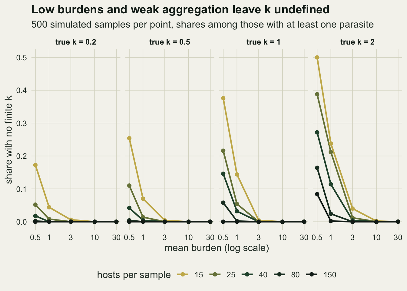
Finite estimates run low only where many are non-finite
Dropping the samples with no finite estimate and summarising the rest is a common first step, if only because a spreadsheet cannot average infinity. The medians below are of the finite estimates only, divided by the true \(k\).
ratio_row <- function(k, what) sapply(mu_set, function(m) cell(25, m, k, what))
ml_hi_small <- cell(15, 0.5, 0.2, "ml_med")
ml_lo_large <- cell(15, 0.5, 2, "ml_med")
ml_lo_large40 <- cell(40, 0.5, 2, "ml_med")
over2_small <- cell(15, 0.5, 0.2, "over2")
mom_range <- range(grid_res$mom_med[grid_res$n <= 40])
ml_big <- range(grid_res$ml_med[grid_res$n == 150 & grid_res$mu >= 3])
mom_big <- range(grid_res$mom_med[grid_res$n == 150 & grid_res$mu >= 3])
mom_above_ml <- mean(grid_res$mom_med > grid_res$ml_med)
mom_low <- grid_res[grid_res$mom_med < 1, ]
mom_low_k <- sort(unique(mom_low$k)); mom_low_mu <- max(mom_low$mu)
mom_k2 <- cell(25, 0.5, 2, "mom_med")
ml_below <- grid_res[grid_res$ml_med < 1, ]
ml_high_nf <- grid_res[grid_res$ml_med >= 1 & grid_res$nonfin >= min(ml_below$nonfin), ]
With fifteen hosts, a mean of 0.5 and a true \(k\) of 0.2, the median finite maximum likelihood estimate is 1.24 times the truth, and 41 per cent of the samples with at least one parasite, counting the infinite ones, report more than twice the true \(k\). Keep the host number and mean and raise the true \(k\) to 2, and the median finite estimate is 0.52 times the truth; at forty hosts it is 0.83. The error runs low only where many samples were lost to infinity: the maximum likelihood median falls below the truth in 7 of the hundred cells, all with a mean of at most 1 and at least 14.6 per cent of samples non-finite; in every other cell, at every \(k\), it is at or above the truth. A large non-finite share is needed but not enough: 4 cells with at least that share still run high, among them the fifteen-host cell at \(k\) = 0.2 above. Where the median does fall, the samples that happen to look aggregated are the ones that yield a finite estimate at all, so the finite ones are selected to be too small, and the ones that would have been too large became infinite instead.
The moment estimator runs high more consistently, but not everywhere. Among the samples of forty hosts or fewer, its finite median runs from 0.80 to 1.83 times the truth, and it sits above the maximum likelihood median in 95 per cent of all hundred cells. It falls below the truth in 7 cells, all with a true \(k\) of 1 or 2 and a mean of at most 1, by the same selection: with twenty five hosts, a mean of 0.5 and \(k\) = 2 its finite median is 0.80 times the truth. With a hundred and fifty hosts and a mean of at least three, both come within about a tenth of the truth: the maximum likelihood medians run from 1.00 to 1.02 times the truth and the moment medians from 1.02 to 1.10.
bias_df <- rbind(
  data.frame(grid_res[grid_res$n == 25, c("mu", "k")], ratio = grid_res$ml_med[grid_res$n == 25],
             estimator = "maximum likelihood"),
  data.frame(grid_res[grid_res$n == 25, c("mu", "k")], ratio = grid_res$mom_med[grid_res$n == 25],
             estimator = "moments"))
bias_df$panel <- factor(paste("true k =", bias_df$k), levels = paste("true k =", k_set))
ggplot(bias_df, aes(mu, ratio, colour = estimator)) +
  geom_hline(yintercept = 1, colour = te_body, linetype = "dashed", linewidth = 0.5) +
  geom_line(linewidth = 0.9) + geom_point(size = 1.8) +
  facet_wrap(~ panel, nrow = 1) +
  scale_x_log10(breaks = mu_set, labels = c("0.5", "1", "3", "10", "30")) +
  scale_colour_manual(values = c(te_forest, te_rust), name = NULL) +
  labs(x = "mean burden (log scale)", y = "median finite estimate / true k",
       title = "Twenty five hosts: the finite estimates",
       subtitle = "dashed line: no bias") +
  theme_datasheet() + theme(legend.position = "bottom")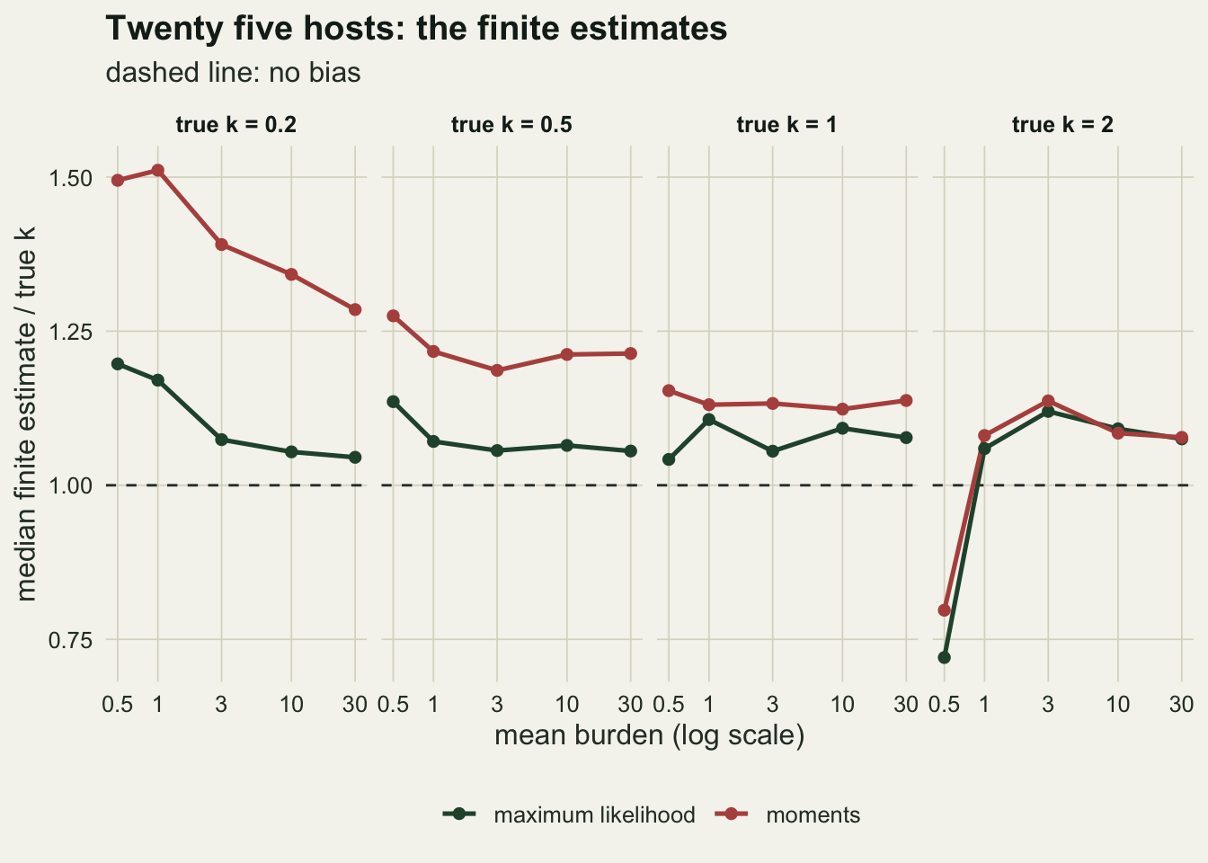
The profile interval says what the point cannot
A point estimate has to be something when the likelihood has no top. An interval does not: it can be open at one end, and the open end is the honest statement that the sample cannot tell weak aggregation from none.
cov_range <- range(grid_res$cover)
cov_low <- grid_res[which.min(grid_res$cover), ]
mcse_cov <- sqrt(0.95 * 0.05 / n_rep_grid)
n_below <- sum(grid_res$cover < 0.95 - 2 * mcse_cov)
open_k2 <- cell(25, 0.5, 2, "open_hi")
open_k05 <- cell(25, 1, 0.5, "open_hi")
w_nonfin <- grid_res$nonfin * (1 - grid_res$all_zero)
cov_nonfin_all <- sum(grid_res$cover_nonfin * w_nonfin, na.rm = TRUE) / sum(w_nonfin)
big_nf <- grid_res$nonfin >= 0.1
cov_nonfin_min <- min(grid_res$cover_nonfin[big_nf])
nf_min_cell <- grid_res[big_nf, ][which.min(grid_res$cover_nonfin[big_nf]), ]
nf_min_count <- n_rep_grid * (1 - nf_min_cell$all_zero) * nf_min_cell$nonfin
nf_min_se <- sqrt(cov_nonfin_min * (1 - cov_nonfin_min) / nf_min_count)
Across the hundred cells the 95 per cent profile interval covers the true \(k\) in between 91.8 and 99.2 per cent of samples. The Monte Carlo standard error near 95 per cent is 1.0 percentage points, and 8 cells fall more than two standard errors below nominal; the lowest is 91.8 per cent, at 25 hosts, a mean of 3 and \(k\) = 0.5. The cost of that coverage is visible in the open intervals. With twenty five hosts at a mean of 0.5 and \(k\) = 2, 91 per cent of the intervals have no upper end; at a mean of 1 and \(k\) = 0.5, 20 per cent. Pooled over the grid, the samples with no finite estimate have the true \(k\) above their lower bound in 85.1 per cent of cases, and in the cells where at least a tenth of samples are non-finite that share goes as low as 66.7 per cent (from about 57 non-finite samples, so give or take 6 points). So given that a sample has no finite estimate, its interval covers less often than nominal; the rates above average over both kinds of sample.
cov_df <- grid_res
cov_df$hosts <- factor(cov_df$n, levels = n_set)
cov_df$kf <- factor(paste("k =", cov_df$k), levels = paste("k =", k_set))
p_cov <- ggplot(cov_df, aes(mu, cover, colour = kf)) +
  annotate("rect", xmin = 0.4, xmax = 38, ymin = 0.95 - 2 * mcse_cov, ymax = 0.95 + 2 * mcse_cov,
           fill = te_line, alpha = 0.7) +
  geom_hline(yintercept = 0.95, colour = te_body, linetype = "dashed", linewidth = 0.5) +
  geom_point(size = 1.9, alpha = 0.85, position = position_jitter(width = 0.04, height = 0, seed = 7)) +
  scale_x_log10(breaks = mu_set, labels = c("0.5", "1", "3", "10", "30")) +
  scale_colour_manual(values = c(te_gold, te_forest, te_rust, te_ink), guide = "none") +
  scale_y_continuous(limits = c(0.85, 1)) +
  labs(x = "mean burden (log scale)", y = "coverage of true k",
       title = "Coverage", subtitle = "band: two MC SE around 0.95") +
  theme_datasheet() + theme(legend.position = "bottom")
p_open <- ggplot(cov_df[cov_df$n == 25, ], aes(mu, open_hi, colour = kf)) +
  geom_line(linewidth = 0.9) + geom_point(size = 1.9) +
  scale_x_log10(breaks = mu_set, labels = c("0.5", "1", "3", "10", "30")) +
  scale_colour_manual(values = c(te_gold, te_forest, te_rust, te_ink), name = "true") +
  scale_y_continuous(limits = c(0, 1)) +
  labs(x = "mean burden (log scale)", y = "share with no upper bound",
       title = "Open intervals, 25 hosts", subtitle = "the price of that coverage") +
  theme_datasheet() + theme(legend.position = "bottom")
p_cov + p_open + plot_layout(guides = "collect") +
  plot_annotation(theme = theme_datasheet()) & theme(legend.position = "bottom")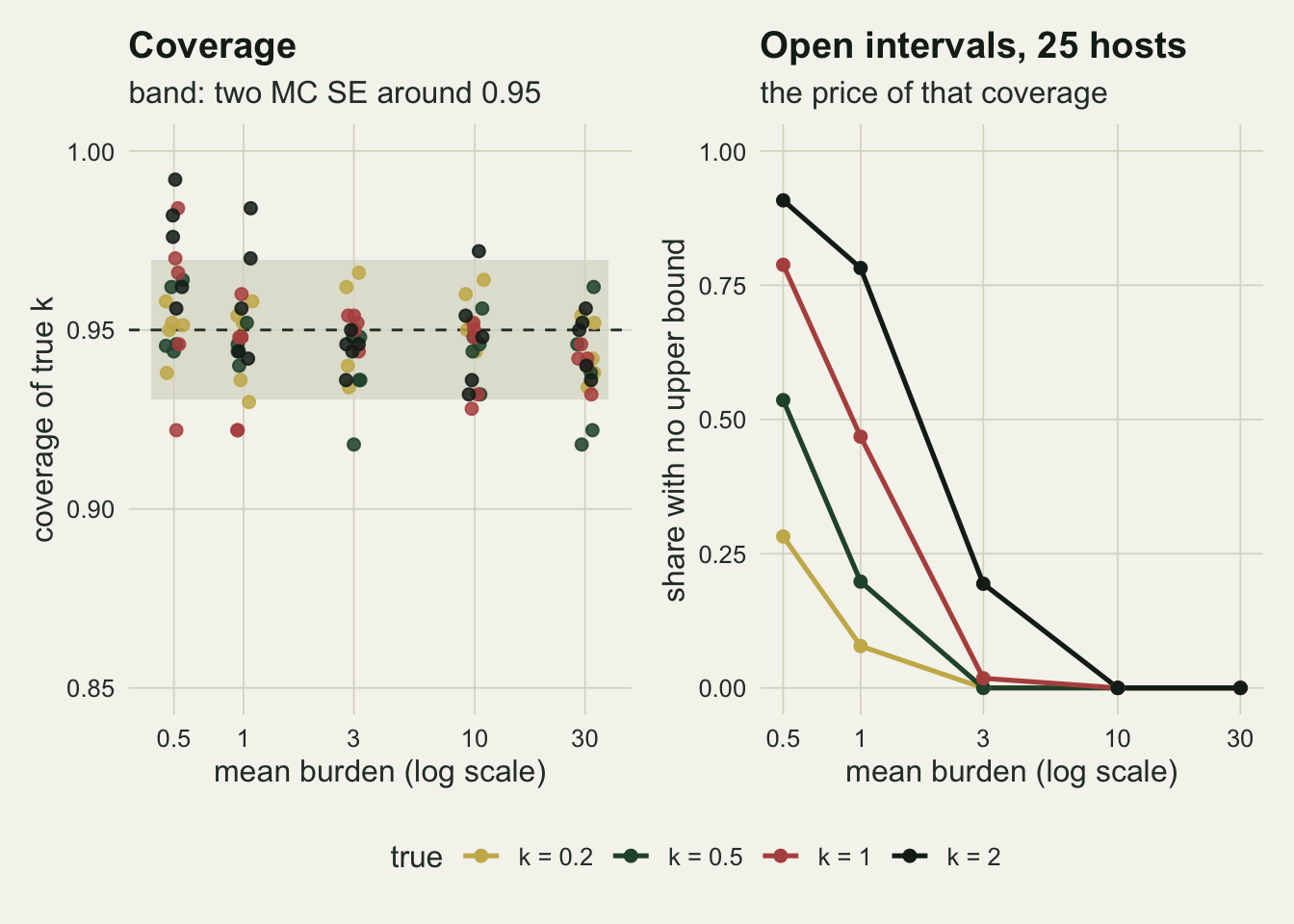
Twenty host groups with one true k
Now the comparison. Twenty lakes, twenty five fish from each, mean burdens spaced evenly on a log scale from 0.3 to 30, and one true \(k\) of 0.5 in every lake. There is no relationship between aggregation and burden to find. Each simulated study regresses \(\log \hat k\) on the log of the sample mean and tests the slope at 5 per cent, under three reporting rules for the lakes with no finite estimate: drop them, record them at a cap of \(k\) = 100 as not aggregated, or report the lower end of the profile interval for every lake. All three rules, the cap and the lake design were fixed before the run.
A fourth analysis needs no rule. It fits every lake in one likelihood, with each lake’s mean at its sample mean and \(\log k\) a straight line in the centred log mean, and tests the slope with a likelihood ratio on one degree of freedom. A lake with its variance below its mean simply contributes a likelihood that prefers large \(k\), like any other observation.
n_lake <- 20; n_fish <- 25; k_common <- 0.5; k_cap <- 100
lake_mu <- exp(seq(log(0.3), log(30), length.out = n_lake))
n_rep_lake <- 1000

nll_joint <- function(par, tabs, z) {
  -sum(vapply(seq_along(tabs), function(j)
    ll_tab(tabs[[j]]$ux, tabs[[j]]$wt, exp(par[1] + par[2] * z[j]), tabs[[j]]$m), 0))
}
joint_test <- function(xs, z) {
  tabs <- lapply(xs, function(x) { tb <- table(x)
    list(ux = as.numeric(names(tb)), wt = as.vector(tb), m = mean(x)) })
  f1 <- optim(c(log(k_common), 0), nll_joint, tabs = tabs, z = z, method = "BFGS")
  f0 <- optimize(function(a) nll_joint(c(a, 0), tabs, z), c(-8, 8))
  c(slope = f1$par[2], lrt = 2 * (f0$objective - f1$value))
}
slope_test <- function(y, x) {
  cf <- summary(lm(log(y) ~ x))$coefficients
  c(cf[2, 1], cf[2, 4] < 0.05)
}
one_study <- function(slope_true = 0) {
  lmu <- log(lake_mu)
  k_lake <- exp(log(k_common) + slope_true * (lmu - mean(lmu)))
  xs <- lapply(seq_len(n_lake), function(j) rnbinom(n_fish, size = k_lake[j], mu = lake_mu[j]))
  fk <- t(sapply(xs, fit_k)); keep <- fk[, "m"] > 0
  xs <- xs[keep]; fk <- fk[keep, , drop = FALSE]
  lsm <- log(fk[, "m"]); fin <- is.finite(fk[, "ml"])
  low_lake <- lake_mu[keep] < 1
  jt <- joint_test(xs, lsm - mean(lsm))
  out <- c(sum(keep), sum(!fin), sum(!fin & low_lake), sum(fin & fk[, "ml"] > 20), sum(fin & fk[, "ml"] > 20 & low_lake),
           slope_test(fk[fin, "ml"], lsm[fin]),
           slope_test(pmin(fk[, "ml"], k_cap), lsm),
           slope_test(pmin(fk[, "ml"], 20), lsm)[2],
           slope_test(pmin(fk[, "ml"], 1000), lsm)[2],
           slope_test(fk[, "lo"], lsm),
           jt[1], jt[2] > qchisq(0.95, 1))
  names(out) <- c("lakes", "nonfin", "nonfin_low", "big_fin", "big_fin_low", "drop1", "drop2", "cap1", "cap2", "cap20", "cap1000",
                  "lower1", "lower2", "joint1", "joint2")
  out
}
set.seed(4104)
studies <- t(replicate(n_rep_lake, one_study()))
st_med <- apply(studies, 2, median); st_mean <- colMeans(studies)
mcse_rej <- sqrt(0.05 * 0.95 / n_rep_lake)
share_any_nonfin <- mean(studies[, "nonfin"] > 0)
lakes_dropped <- sum(studies[, "lakes"] < n_lake)
share_nf_low <- sum(studies[, "nonfin_low"]) / sum(studies[, "nonfin"])
n_low_lakes <- sum(lake_mu < 1)
big_fin_rate <- st_mean["big_fin"]
big_fin_share <- mean(studies[, "big_fin"] > 0)
big_fin_low_share <- sum(studies[, "big_fin_low"]) / sum(studies[, "big_fin"])
In 50 per cent of the 1000 simulated studies at least one lake has no finite estimate, with 0.63 such lakes per study on average, and 96.0 per cent of those lakes are among the 5 whose true mean is below one fluke per fish. (A lake in which every fish was clean would have no mean to regress on and was removed from all four analyses; that happened in 3 studies.)
Recording those lakes at the cap gives a median slope of -0.22 and declares a relationship between aggregation and burden in 28.7 per cent of studies: low-burden lakes look less aggregated, and none of it is real. The size of the cap barely matters to the verdict, 27.6 per cent at a cap of 20 and 28.4 per cent at 1000. Reporting the lower profile bound turns the pattern around: median slope +0.24, a significant slope in 78.8 per cent of studies, and the low-burden lakes now look more aggregated, since a sample with little information has a lower bound far below any central value. Dropping the lakes gives a median slope of -0.04, but the regression still rejects in 11.0 per cent of studies against a nominal 5, with a Monte Carlo standard error of 0.7 points. Two things feed that excess and the simulation does not separate them. A lake whose variance lies just above its mean gets a finite but huge estimate: a finite \(\hat k\) above 20, forty times the truth, turns up in 13 per cent of studies (0.14 lakes per study), and 95 per cent of those lakes have a true mean below one, the same pull the cap exerts; and a \(\log \hat k\) from a lake at a mean of 0.3 is far noisier than one at 30 while the ordinary regression weights them equally.
The joint likelihood has a median slope of -0.026 and rejects in 4.7 per cent of studies, within Monte Carlo error of nominal.
slope_alt <- 0.3
n_rep_alt <- 300
set.seed(4105)
alt <- t(replicate(n_rep_alt, one_study(slope_true = slope_alt)))
alt_mean <- colMeans(alt); alt_med <- apply(alt, 2, median)
mcse_pow <- sqrt(alt_mean["joint2"] * (1 - alt_mean["joint2"]) / n_rep_alt)
Given a real relationship, with \(\log k\) rising by 0.3 for each unit of log mean, the joint likelihood detects it in 91 per cent of 300 studies (Monte Carlo standard error 1.7 points), with a median slope estimate of 0.25. The drop rule detects it in 61 per cent with a median slope of 0.22. Both medians sit below the true 0.3, as expected when the covariate is itself a noisy sample mean.
rule_lev <- c("cap at 100", "lower profile bound", "drop non-finite", "joint likelihood")
sl_df <- data.frame(rule = factor(rep(rule_lev, each = n_rep_lake), levels = rev(rule_lev)),
                    slope = c(studies[, "cap1"], studies[, "lower1"], studies[, "drop1"],
                              studies[, "joint1"]))
rej_df <- data.frame(rule = factor(rule_lev, levels = rev(rule_lev)),
                     rate = c(st_mean["cap2"], st_mean["lower2"], st_mean["drop2"], st_mean["joint2"]))
rule_cols <- c("cap at 100" = te_rust, "lower profile bound" = te_gold,
               "drop non-finite" = te_forest, "joint likelihood" = te_ink)
p_sl <- ggplot(sl_df, aes(slope, rule, fill = rule)) +
  geom_vline(xintercept = 0, colour = te_body, linetype = "dashed", linewidth = 0.5) +
  geom_boxplot(width = 0.55, outlier.size = 0.6, outlier.alpha = 0.4, colour = te_ink, alpha = 0.55,
               linewidth = 0.4) +
  scale_fill_manual(values = rule_cols, guide = "none") +
  coord_cartesian(xlim = c(-1, 1)) +
  labs(x = "slope of log k on log mean", y = NULL, title = "Estimated slope",
       subtitle = "dashed line: the true slope of zero") +
  theme_datasheet()
p_rej <- ggplot(rej_df, aes(rate, rule, fill = rule)) +
  geom_col(width = 0.55) +
  geom_vline(xintercept = 0.05, colour = te_body, linetype = "dashed", linewidth = 0.5) +
  scale_fill_manual(values = rule_cols, guide = "none") +
  scale_x_continuous(limits = c(0, 1)) +
  labs(x = "share significant", y = NULL, title = "False relationships",
       subtitle = "dashed line: 5 per cent") +
  theme_datasheet() + theme(axis.text.y = element_blank())
p_sl + p_rej + plot_layout(widths = c(1.4, 1)) + plot_annotation(theme = theme_datasheet())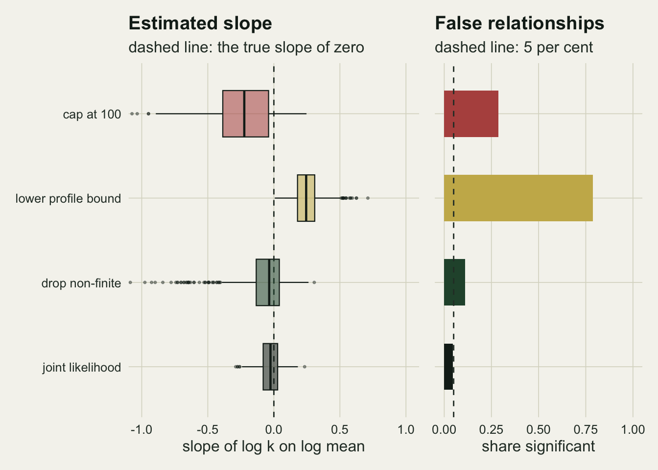
What to report
Give the number of hosts and the mean burden next to every \(k\). They decide how often \(k\) is undefined, and a reader cannot judge a \(k\) from twenty five fish without them.
When the variance does not exceed the mean, say so in those words and report the profile interval with its open upper end. Do not substitute a large number, and do not silently leave the sample out of a table that is later compared across groups. Across all samples the interval’s coverage stayed between 91.8 and 99.2 per cent, but for the non-finite samples alone the lower bound held in only 85.1 per cent, so treat that lower bound as optimistic. It is still the only defensible statement from such a sample; the point estimate has nothing to offer. If a table needs a single entry, Lloyd-Smith’s convention of an infinite \(k\) is honest, provided the table says so and is not then fed to a regression.
State the variance divisor used for the rule, or report both variances. In a small share of samples the two rules disagree, and the moment and maximum likelihood estimates then fall on different sides of the line.
To compare aggregation across host groups, fit the groups in one likelihood with \(k\) modelled as a function of the group covariate, rather than regressing a column of separately estimated \(k\) values. That is the analysis that held its error rate here, and it needs no rule for the awkward samples.
Honest limits
Every sample here is a genuine negative binomial with a known \(k\). Real burden distributions are often mixtures, zero-inflated, or truncated by host death as in the neighbouring post, and a sample whose variance falls below its mean can also mean that the negative binomial is the wrong family for it. Nothing above separates those cases.
The comparative act uses one design: twenty groups, twenty five hosts each, a common \(k\) of 0.5 and means spread evenly on a log scale from 0.3 to 30. The false relationship under the cap rule depends on how many groups sit at low burdens. The non-finite share that drives it rises with \(k\) and falls with host number, so a compilation of large samples, or of strongly aggregated parasites with few low-burden groups, would show less of it; neither was simulated.
The joint likelihood used the sample mean as the covariate for \(k\), which is also the fitted mean in the same likelihood; because that covariate is noisy, slope estimates under the alternative were attenuated, for the joint likelihood as for the drop rule. Its error rate was measured at one design and its power at one alternative slope, with 300 studies; a parametric bootstrap of the likelihood ratio would be the safer reference if the group count or host number were much smaller.
Only the moment and maximum likelihood estimators were compared. Corrected moment forms, the zero-class estimator and Bayesian fits with a prior on \(1/k\) behave differently when the likelihood has no top; a prior turns the open interval into a closed one whose upper end is set by the prior, which should then be reported as such.
The grid used 500 samples per cell, so shares and coverages carry Monte Carlo standard errors up to the values quoted above; cell-to-cell wiggles smaller than two of them in the figures are noise.
References
Pieters EP, Gates CE, Matis JH, Sterling WL 1977 Biometrics 33(4):718 (10.2307/2529470)
Gregory RD, Woolhouse MEJ 1993 Acta Tropica 54(2):131-139 (10.1016/0001-706X(93)90059-K)
Shaw DJ, Dobson AP 1995 Parasitology 111(S1):S111-S133 (10.1017/S0031182000075855)
Lloyd-Smith JO 2007 PLoS ONE 2(2):e180 (10.1371/journal.pone.0000180)