---
title: "Simulating correlated variables in R"
description: "Simulate correlated variables in R by hand, with chol() and with mvrnorm(), and why a correlation set on the log scale is not the correlation of the counts."
date: "2026-09-28 08:00"
categories: [R, simulation, statistics, count data, ecology tutorial]
image: thumbnail.png
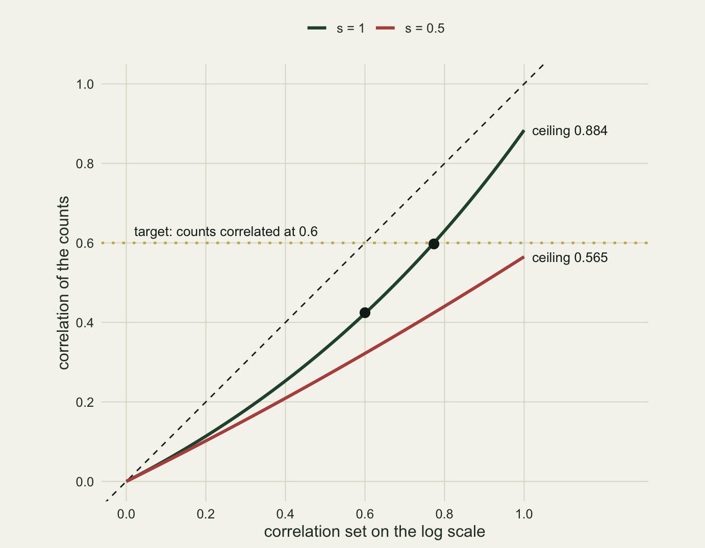
image-alt: "Line chart with the correlation set on the log scale on the horizontal axis from 0 to 1 and the correlation of the counts on the vertical axis from 0 to 1. A dashed black diagonal marks where the two are equal and a dotted gold horizontal line at 0.6 is labelled target: counts correlated at 0.6. A dark green curve for s = 1 starts at 0, bends upward below the diagonal and ends at 0.884, labelled ceiling 0.884. A red curve for s = 0.5 runs below it, almost straight, and ends at 0.565, labelled ceiling 0.565, below the target line. Two black points sit on the green curve, one above 0.6 on the horizontal axis at about 0.42, and one at about 0.77 where the green curve meets the target line."
---
A pilot survey counted two ground beetle species in pitfall traps at 40 grassland sites. The first species averaged a few beetles per trap, the second several more, and sites that were good for one tended to be good for the other: the Pearson correlation between the two columns of counts was about 0.6. The next step is a power analysis for a larger survey, and that needs simulated surveys that look like the pilot, with the two species correlated as they were in the field. How do you simulate two correlated variables, and how do you make the counts come out correlated at 0.6?
[Power analysis by simulation in R](../power-analysis-by-simulation/) builds the simulation loop, the approach Bolker (2008) teaches for ecological models, and [Probability distributions in R: d, p, q and r](../probability-distributions-in-r/) explains `rnorm()` and `rpois()`. Neither makes two variables move together. Dozens of posts on this site do, usually with one line built around `chol()` or `MASS::mvrnorm()` and no comment. This post explains that line, then measures the trap that is easy to walk into the first time you simulate correlated counts.
**The short answer.** Draw independent standard normals and mix them: for two variables, `x2 <- rho * z1 + sqrt(1 - rho^2) * z2`; for any number, `Z %*% chol(Sigma)`, with the Cholesky factor on the right of the matrix of draws, or let `MASS::mvrnorm()` do it. For counts, the usual route puts the correlation on a hidden log scale and draws Poisson counts from it. The counts then correlate less than the number you typed, so decide first which scale your target belongs to. If it is the correlation of the counts, solve for the log-scale value that produces it, and check that it can be produced at all.
All data here are simulated, and every seed is in the code.
```{r setup}
#| message: false
library(ggplot2)

te_paper  <- "#f5f4ee"
te_ink    <- "#16241d"
te_body   <- "#2c3a31"
te_forest <- "#275139"
te_rust   <- "#b5534e"
te_gold   <- "#c9b458"
te_line   <- "#dad9ca"

theme_datasheet <- function() {
  theme_minimal(base_size = 12) +
    theme(plot.background  = element_rect(fill = te_paper, colour = NA),
          panel.background = element_rect(fill = te_paper, colour = NA),
          panel.grid.major = element_line(colour = te_line, linewidth = 0.3),
          panel.grid.minor = element_blank(),
          text             = element_text(colour = te_body),
          axis.text        = element_text(colour = te_body),
          strip.text       = element_text(colour = te_ink, face = "bold"))
}
```
## Two correlated variables by hand
Start with two independent standard normals, `z1` and `z2`. Keep `z1` as the first variable and build the second from both: a share `rho` of `z1` plus enough of `z2` to bring the variance back to one.
```{r two-by-hand}
set.seed(1015)
n_big <- 1e5
rho   <- 0.6

z1 <- rnorm(n_big)
z2 <- rnorm(n_big)
x1 <- z1
x2 <- rho * z1 + sqrt(1 - rho^2) * z2

round(c(sd_x1 = sd(x1), sd_x2 = sd(x2), correlation = cor(x1, x2)), 3)
```
```{r two-numbers}
#| include: false
cor_by_hand <- cor(x1, x2)
stopifnot(isTRUE(all.equal(cor(x1, 10 + 2 * x2), cor_by_hand)))
```
The algebra is two lines. The variance of `x2` is `rho^2 + (1 - rho^2) = 1`, because `z1` and `z2` are independent with variance one, and the covariance of `x1` and `x2` is `rho`, because only the `z1` part is shared. Both standard deviations are one, so the covariance is also the correlation, and a hundred thousand draws give `r sprintf("%.3f", cor_by_hand)` against the `r rho` we asked for. To give the variables other means and spreads, multiply and add afterwards: `10 + 2 * x2` has correlation `rho` with `x1` too, because shifting and rescaling does not change a correlation.
## Any number of variables: chol()
With three or more variables the mixing weights are no longer obvious, and the Cholesky decomposition supplies them. Say three species have log-abundances that correlate at 0.6, 0.3 and 0.5 in pairs. Write the targets into a correlation matrix and hand it to `chol()`:
```{r chol-three}
sigma3 <- matrix(c(1.0, 0.6, 0.3,
                   0.6, 1.0, 0.5,
                   0.3, 0.5, 1.0), nrow = 3)
chol_upper <- chol(sigma3)
round(chol_upper, 3)
```
```{r chol-guard}
#| include: false
# chol() returns the UPPER triangular factor R, with t(R) %*% R equal to the matrix
stopifnot(all(chol_upper[lower.tri(chol_upper)] == 0),
isTRUE(all.equal(t(chol_upper) %*% chol_upper, sigma3)),
isTRUE(all.equal(chol_upper[, 1], c(1, 0, 0))),
isTRUE(all.equal(chol_upper[1:2, 2], c(0.6, sqrt(1 - 0.6^2)))))
```
`chol()` returns an upper triangular matrix, zeros below the diagonal, and it is the factor `R` for which `t(R) %*% R` gives back `sigma3`. That orientation decides which side of the draws it goes on. Put independent standard normals in a matrix with one row per site and one column per variable, and multiply by `R` on the right:
```{r chol-draw}
set.seed(2015)
z3 <- matrix(rnorm(3 * n_big), ncol = 3)
x3 <- z3 %*% chol_upper
round(cor(x3), 3)
```
The covariance of `z3 %*% R` is `t(R) %*% R`, which is `sigma3`, and the simulated correlations match the targets. The first column of `R` is `(1, 0, 0)`, so the first variable is simply the first column of draws, and the second column of `R` holds the same two weights as the hand-made `x2` above: the by-hand recipe is the two-variable Cholesky factor written out.
Put the factor on the other side, `z3 %*% t(R)`, and the covariance becomes `R %*% t(R)`, which is a different matrix:
```{r chol-wrong}
x3_wrong <- z3 %*% t(chol_upper)
round(cor(x3_wrong), 3)
round(diag(var(x3_wrong)), 3)
```
```{r chol-wrong-numbers}
#| include: false
wrong_cor3 <- cor(x3_wrong)
wrong_exact3 <- cov2cor(chol_upper %*% t(chol_upper))
wrong_var3 <- diag(var(x3_wrong))
chol2 <- chol(matrix(c(1, rho, rho, 1), 2))
wrong_exact2 <- cov2cor(chol2 %*% t(chol2))[1, 2]
stopifnot(isTRUE(all.equal(wrong_exact2, rho / sqrt(1 + rho^2))))
# a single draw as a column vector: t(R) %*% z is the same product, transposed
stopifnot(isTRUE(all.equal(t(z3[1:5, ] %*% chol_upper), t(chol_upper) %*% t(z3[1:5, ]))))
```
The targets 0.6, 0.3 and 0.5 come out as `r sprintf("%.3f", wrong_cor3[1, 2])`, `r sprintf("%.3f", wrong_cor3[1, 3])` and `r sprintf("%.3f", wrong_cor3[2, 3])`, and the variances, which should all be one, run from `r sprintf("%.2f", min(wrong_var3))` to `r sprintf("%.2f", max(wrong_var3))`. Nothing warns you. The same mistake with only two variables is no safer: `R %*% t(R)` then has correlation `rho / sqrt(1 + rho^2)`, which is `r sprintf("%.3f", wrong_exact2)` for a target of `r rho`. Some posts on this site draw one realisation at a time as a column, `t(chol(Sigma)) %*% z`; that is the correct product for a column, because it is the transpose of `z %*% chol(Sigma)` for a row.
The shortcut is `mvrnorm()` from the MASS package that accompanies Venables and Ripley (2002). It takes the means and the covariance matrix and returns one row per draw:
```{r mvrnorm}
set.seed(3015)
x3_mass <- MASS::mvrnorm(n_big, mu = c(0, 0, 0), Sigma = sigma3)
round(cor(x3_mass), 3)
```
```{r mvrnorm-guard}
#| include: false
# MASS::mvrnorm() factorises Sigma with eigen(), not chol()
stopifnot(any(grepl("eigen(", deparse(body(MASS::mvrnorm)), fixed = TRUE)),
!any(grepl("chol(", deparse(body(MASS::mvrnorm)), fixed = TRUE)))
```
Internally `mvrnorm()` uses an eigen decomposition of `Sigma` rather than `chol()`, so the individual draws differ from the Cholesky ones, but the covariance they are drawn from is the same. It is the line to use in practice; writing the Cholesky version once is what makes it readable.
## Correlated counts: the correlation you set is not the one you get
Now the beetles. Counts are not normal, so the usual route, and the one behind most joint species models for counts, puts the correlation on a hidden scale. Each site gets a pair of correlated normal log-abundances with standard deviation `s`; each species' expected count is its site mean times the exponential of its log-abundance; and the trap catches a Poisson count around that expectation. Subtracting `s^2 / 2` inside the exponential keeps the average count at the site mean, because the mean of `exp(x)` for a normal `x` with mean zero and standard deviation `s` is `exp(s^2 / 2)`.
```{r simulate-counts}
simulate_counts <- function(n_sites, rho_latent, s, mu) {
  sigma  <- s^2 * matrix(c(1, rho_latent, rho_latent, 1), nrow = 2)
  latent <- matrix(rnorm(2 * n_sites), ncol = 2) %*% chol(sigma)
  expected <- cbind(mu[1] * exp(latent[, 1] - s^2 / 2),
                    mu[2] * exp(latent[, 2] - s^2 / 2))
  counts <- matrix(rpois(2 * n_sites, expected), ncol = 2)
  list(latent = latent, counts = counts)
}

mu_beetle <- c(3, 8)   # mean beetles per trap, species A and B
s_log     <- 1         # standard deviation of log-abundance between sites
n_sites   <- 40

set.seed(4015)
survey <- simulate_counts(n_sites, rho_latent = 0.6, s = s_log, mu = mu_beetle)
head(survey$counts)
round(c(latent = cor(survey$latent)[1, 2], counts = cor(survey$counts)[1, 2]), 3)
```
```{r survey-numbers}
#| include: false
survey_latent <- cor(survey$latent)[1, 2]
survey_counts <- cor(survey$counts)[1, 2]
```
In this one simulated survey the log-abundances correlate at `r sprintf("%.3f", survey_latent)` and the counts at `r sprintf("%.3f", survey_counts)`. One survey of 40 sites is noisy, so the chunk below asks what the counts correlate at in the long run: forty batches of fifty thousand sites each, with the correlation computed in every batch and averaged, so that the spread between batches gives a Monte Carlo standard error.
```{r long-run}
long_run <- function(rho_latent, s, mu, n_batch = 40, batch_size = 5e4) {
  per_batch <- replicate(n_batch, {
    sim <- simulate_counts(batch_size, rho_latent, s, mu)
    c(latent    = cor(sim$latent)[1, 2],
      lognormal = cor(exp(sim$latent))[1, 2],
      counts    = cor(sim$counts)[1, 2],
      var_a     = var(sim$counts[, 1]),
      var_b     = var(sim$counts[, 2]),
      cov_ab    = cov(sim$counts)[1, 2])
  })
  rbind(mean = rowMeans(per_batch),
        mc_se = apply(per_batch, 1, sd) / sqrt(n_batch))
}

set.seed(5015)
run_06 <- long_run(0.6, s_log, mu_beetle)
round(run_06, 3)
```
The latent correlation is the `r sprintf("%.2f", run_06["mean", "latent"])` we set. The exponentials of the log-abundances already correlate at only `r sprintf("%.3f", run_06["mean", "lognormal"])`, and the counts at `r sprintf("%.3f", run_06["mean", "counts"])`. A power analysis run with `rho_latent = 0.6` would simulate beetles that are much less tied to each other than the pilot's, and every power figure from it would answer a different question.
None of this needs a simulation to predict. Two short results give the long-run values. The count formulas are in Aitchison and Ho (1989); the first result is the same calculation without the Poisson term. For the exponentials: the sum of the two log-abundances is normal with variance `2 s^2 (1 + rho)`, so the mean of the product of the exponentials is `exp(s^2 (1 + rho))`, and dividing the covariance by the variance gives
```
cor(exp(x1), exp(x2)) = (exp(rho * s^2) - 1) / (exp(s^2) - 1)
```
For the counts: given the expected counts, the two Poisson draws are independent, so the Poisson noise adds its mean to each variance and nothing to the covariance,
```
var(y)       = mu + mu^2 * (exp(s^2) - 1)
cov(y1, y2)  = mu1 * mu2 * (exp(rho * s^2) - 1)
```
and the count correlation is the covariance over the product of the two standard deviations. The Poisson term `mu` in each variance is the second loss: it is largest, relative to the rest, for the rarer species.
```{r closed-form}
count_cor <- function(rho_latent, s, mu) {
  cov_ab <- mu[1] * mu[2] * (exp(rho_latent * s^2) - 1)
  var_ab <- mu + mu^2 * (exp(s^2) - 1)
  cov_ab / sqrt(var_ab[1] * var_ab[2])
}
closed <- c(lognormal = (exp(0.6 * s_log^2) - 1) / (exp(s_log^2) - 1),
            counts    = count_cor(0.6, s_log, mu_beetle),
            var_a     = mu_beetle[1] + mu_beetle[1]^2 * (exp(s_log^2) - 1),
            var_b     = mu_beetle[2] + mu_beetle[2]^2 * (exp(s_log^2) - 1),
            cov_ab    = prod(mu_beetle) * (exp(0.6 * s_log^2) - 1))
z_scores <- (run_06["mean", names(closed)] - closed) / run_06["mc_se", names(closed)]
round(rbind(closed = closed, simulated = run_06["mean", names(closed)], z = z_scores), 3)
```
```{r closed-guard}
#| include: false
stopifnot(all(abs(z_scores) < 3))
```
Each simulated value is within `r sprintf("%.1f", ceiling(10 * max(abs(z_scores))) / 10)` Monte Carlo standard errors of its formula: the loss from `r sprintf("%.2f", 0.6)` to `r sprintf("%.3f", closed["counts"])` is arithmetic, not a finding of the simulation. It depends only on `rho`, `s` and the two means.
The pilot's own 0.6 has a second weakness: it comes from 40 sites. Here is the spread of the count correlation across four thousand simulated 40-site surveys, all with the same log-scale correlation of 0.6:
```{r forty-sites}
set.seed(6015)
cor_40 <- replicate(4000, {
  cor(simulate_counts(n_sites, 0.6, s_log, mu_beetle)$counts)[1, 2]
})
round(quantile(cor_40, c(0.10, 0.50, 0.90)), 3)
```
```{r forty-numbers}
#| include: false
q_40 <- quantile(cor_40, c(0.10, 0.50, 0.90))
share_40_above <- mean(cor_40 >= 0.6)
```
The long-run count correlation of this design is `r sprintf("%.3f", closed["counts"])`, yet one survey in ten reports less than `r sprintf("%.3f", q_40[1])` and one in ten more than `r sprintf("%.3f", q_40[3])`, with the middle survey at `r sprintf("%.3f", q_40[2])`; `r sprintf("%.1f", 100 * share_40_above)` per cent of these surveys report 0.6 or more. A pilot value of 0.6 from 40 sites can therefore come from a process whose long-run count correlation is well below 0.6, which is worth remembering whichever scale you settle on.
## The fix: decide which scale the target lives on
If your 0.6 is a correlation on the log scale, for example a residual correlation from a fitted Poisson or negative binomial mixed model or a joint species model, then `rho_latent = 0.6` is already right and the counts should correlate less. If it is the Pearson correlation of the raw counts, as in the pilot, solve for the log-scale value that produces it. `count_cor()` rises steadily with `rho_latent`, so `uniroot()` can search between 0 and 1:
```{r solve-rho}
target <- 0.6
rho_needed <- uniroot(function(r) count_cor(r, s_log, mu_beetle) - target,
                      interval = c(0, 1))$root
rho_needed
set.seed(7015)
run_fixed <- long_run(rho_needed, s_log, mu_beetle)
round(run_fixed[, c("latent", "counts")], 3)
```
```{r solve-numbers}
#| include: false
z_fixed <- (run_fixed["mean", "counts"] - target) / run_fixed["mc_se", "counts"]
```
A log-scale correlation of `r sprintf("%.3f", rho_needed)` gives counts that correlate at `r sprintf("%.3f", run_fixed["mean", "counts"])` in the long run (Monte Carlo standard error `r sprintf("%.3f", run_fixed["mc_se", "counts"])`), `r sprintf("%.1f", abs(z_fixed))` standard errors from the target. That is the number to put into the power analysis.
There is a limit, and it is better to see it before calling `uniroot()`. Even with `rho_latent = 1`, when both species follow exactly the same log-abundance, the Poisson noise keeps the counts apart, so the count correlation has a ceiling. The ceiling depends on how much the sites differ, `s`, and on how large the counts are: what matters is the between-site variance `mu^2 * (exp(s^2) - 1)` against the Poisson variance `mu`, so rarer species and more similar sites both lower it:
```{r ceiling}
ceiling_s1  <- count_cor(1, s = 1,   mu = mu_beetle)
ceiling_s05 <- count_cor(1, s = 0.5, mu = mu_beetle)
ceiling_s05_x10 <- count_cor(1, s = 0.5, mu = 10 * mu_beetle)
round(c(ceiling_s1 = ceiling_s1, ceiling_s05 = ceiling_s05, ceiling_s05_x10 = ceiling_s05_x10), 3)
no_root <- tryCatch(
  uniroot(function(r) count_cor(r, 0.5, mu_beetle) - target, interval = c(0, 1)),
  error = function(e) conditionMessage(e))
no_root
```
```{r ceiling-guard}
#| include: false
floor_s1 <- count_cor(-1, s = 1, mu = mu_beetle)
stopifnot(ceiling_s05 < target, ceiling_s1 > target, ceiling_s05_x10 > target, floor_s1 > -1,
is.character(no_root), grepl("opposite sign", no_root))
```
With `s = 1` the counts can reach `r sprintf("%.3f", ceiling_s1)`, so 0.6 is attainable. With `s = 0.5`, sites that differ less, and these small means, the ceiling is `r sprintf("%.3f", ceiling_s05)`: no log-scale correlation gives counts correlated at 0.6, and `uniroot()` stops with the message above, because the function it searches is below zero at both ends of the interval. That error is the model telling you the target is impossible, not a numerical problem to work around. If you meet it, either the pilot correlation is higher than this kind of process can produce (and with 40 sites, the previous section shows how easily that happens), or the counts vary between sites more than your `s` says. The same `s = 0.5` with means ten times larger, `r 10 * mu_beetle[1]` and `r 10 * mu_beetle[2]` beetles per trap, lifts the ceiling to `r sprintf("%.3f", ceiling_s05_x10)`, because the Poisson noise then matters much less.
```{r fig-count-cor}
#| echo: false
#| fig-width: 7.2
#| fig-height: 5.6
#| fig-cap: "Long-run correlation of two simulated Poisson counts (site means 3 and 8) against the correlation set on the log scale, for a between-site log-scale standard deviation of 1 and of 0.5, from the closed form. The dashed line is where the two would be equal. Points are the simulated long-run values at a log-scale correlation of 0.6 and at the value solved for a count correlation of 0.6 (dotted line). Each curve ends at its ceiling, the count correlation when the log-scale correlation is 1."
#| fig-alt: "Line chart with the correlation set on the log scale on the horizontal axis from 0 to 1 and the correlation of the counts on the vertical axis from 0 to 1. A dashed black diagonal marks where the two are equal and a dotted gold horizontal line at 0.6 is labelled target: counts correlated at 0.6. A dark green curve for s = 1 starts at 0, bends upward below the diagonal and ends at 0.884, labelled ceiling 0.884. A red curve for s = 0.5 runs below it, almost straight, and ends at 0.565, labelled ceiling 0.565, below the target line. Two black points sit on the green curve, one above 0.6 on the horizontal axis at about 0.42, and one at about 0.77 where the green curve meets the target line."
curve_grid <- expand.grid(rho_latent = seq(0, 1, by = 0.01), s = c(1, 0.5))
curve_grid$count_cor <- mapply(count_cor, curve_grid$rho_latent, curve_grid$s,
MoreArgs = list(mu = mu_beetle))
curve_grid$s_label <- factor(ifelse(curve_grid$s == 1, "s = 1", "s = 0.5"), levels = c("s = 1", "s = 0.5"))
ceiling_labels <- data.frame(rho_latent = 1.02, count_cor = c(ceiling_s1, ceiling_s05),
label = sprintf("ceiling %.3f", c(ceiling_s1, ceiling_s05)))
sim_points <- data.frame(rho_latent = c(0.6, rho_needed),
count_cor = c(run_06["mean", "counts"], run_fixed["mean", "counts"]))
ggplot(curve_grid, aes(rho_latent, count_cor)) +
geom_abline(intercept = 0, slope = 1, linetype = "dashed", colour = te_ink, linewidth = 0.5) +
geom_hline(yintercept = target, linetype = "dotted", colour = te_gold, linewidth = 0.9) +
geom_line(aes(colour = s_label), linewidth = 1.1) +
geom_point(data = sim_points, size = 3, colour = te_ink) +
geom_text(data = ceiling_labels, aes(label = label), hjust = 0, size = 3.5,
colour = te_ink) +
annotate("text", x = 0.02, y = target + 0.03, hjust = 0, size = 3.5, colour = te_ink,
label = "target: counts correlated at 0.6") +
scale_colour_manual(values = c("s = 1" = te_forest, "s = 0.5" = te_rust)) +
scale_x_continuous(limits = c(0, 1.25), breaks = seq(0, 1, 0.2)) +
scale_y_continuous(limits = c(0, 1), breaks = seq(0, 1, 0.2)) +
coord_equal() +
labs(x = "correlation set on the log scale", y = "correlation of the counts", colour = NULL) +
theme_datasheet() +
theme(legend.position = "top")
```
## What to check in your own data
Check the orientation once, on a large draw: `round(cor(Z %*% chol(Sigma)), 2)` should reproduce your target matrix, and the variances should be the diagonal of `Sigma`. If they are not, the factor is on the wrong side.
Write down which scale your target correlation was measured on. A residual correlation from a mixed model or a joint species model lives on the link scale; a correlation of raw counts lives on the count scale. Simulating one as if it were the other is the mistake measured above. [Checking a joint species distribution model](../checking-a-jsdm/) goes the other way for presence-absence data, reading a latent correlation back from a two by two table with the tetrachoric correlation.
Estimate `s` from the pilot before you solve for the log-scale correlation. For each species, the variance formula above rearranges to `s^2 = log(1 + (var(y) - mean(y)) / mean(y)^2)`; if the variance is not above the mean, the counts show no extra spread between sites, `s` is near zero and so is any count correlation this model can make. If the two species give different values, the covariance becomes `mu1 * mu2 * (exp(rho * s1 * s2) - 1)` with `s1^2` and `s2^2` in the two variances.
Compare the ceiling, `count_cor(1, s, mu)`, with your target before calling `uniroot()`. Then simulate a large batch at the solved value and check the counts hit the target. [Testing your analysis code](../testing-your-analysis-code/) shows how to keep a check like that as a test that runs every time the simulator changes.
## Honest limits
The count model here is Poisson on a lognormal, with one `s` for both species; a negative binomial simulator, or a zero-inflated one, has other formulas and another ceiling, although the same `uniroot()` approach works once the formula is written down, or with a simulated long run in its place. Only positive correlations were shown, and a negative target meets a floor as well: at `s = 1` and these two means, `count_cor(-1, 1, mu)` is `r sprintf("%.3f", floor_s1)`, so the counts cannot correlate more negatively than that. The whole post is about the Pearson correlation of two counts, which is only one summary of how two species go together; [Copulas for dependent ecological data](../copulas-for-dependent-ecological-data/) measures the limits that any pair of marginal distributions puts on it, and [Co-occurrence is not interaction](../co-occurrence-is-not-interaction/) explains why a correlation between two species, on either scale, says nothing on its own about why they go together. Finally, the pilot correlation is itself uncertain, as the 40-site spread showed, so a power analysis that is sensitive to it should be run over a range of plausible correlations, not at one solved value, and over a range of `s`, which a 40-site pilot also pins down only loosely.
## References
Aitchison J, Ho CH 1989 Biometrika 76(4):643-653 (10.1093/biomet/76.4.643)
Bolker BM 2008 Ecological Models and Data in R (ISBN 9780691125220)
Venables WN, Ripley BD 2002 Modern Applied Statistics with S, 4th edition (ISBN 9780387954578)
## Related tutorials
- [Power analysis by simulation in R](../power-analysis-by-simulation/)
- [Probability distributions in R: d, p, q and r](../probability-distributions-in-r/)
- [Copulas for dependent ecological data](../copulas-for-dependent-ecological-data/)
- [Checking a joint species distribution model](../checking-a-jsdm/)