library(ggplot2)
library(patchwork)

te_paper  <- "#f5f4ee"
te_ink    <- "#16241d"
te_body   <- "#2c3a31"
te_forest <- "#275139"
te_rust   <- "#b5534e"
te_gold   <- "#c9b458"
te_line   <- "#dad9ca"

theme_datasheet <- function() {
  theme_minimal(base_size = 12) +
    theme(plot.background  = element_rect(fill = te_paper, colour = NA),
          panel.background = element_rect(fill = te_paper, colour = NA),
          panel.grid.major = element_line(colour = te_line, linewidth = 0.3),
          panel.grid.minor = element_blank(),
          text             = element_text(colour = te_body),
          plot.title       = element_text(colour = te_ink, face = "bold"),
          plot.subtitle    = element_text(colour = te_body),
          axis.text        = element_text(colour = te_body))
}Correlations from gradients of different length
R
meta-analysis
effect size
heterogeneity
simulation
ecology tutorial
Studies that share one slope but sample gradients of different length give heterogeneous correlations. Simulating the meta-analysis in R, and two repairs.
A synthesis of leaf mass per area against elevation collects twenty field studies. Each one ran a transect, measured the trait on a few dozen plants and reported a Pearson correlation, because a correlation is the effect size that every paper can be made to yield. The transects are not alike. A study in a small reserve covered a few hundred metres of elevation; a study along a mountain range covered more than a thousand. Suppose the plants are the same everywhere: the trait changes by the same amount per metre in every study and scatters around that line by the same amount. The twenty correlations will still differ, and they will differ in step with how much elevation each study covered.
That is an old result and this post is a demonstration of it, not a claim to it. Greenland, Schlesselman and Criqui 1986 set out why a correlation or a standardised coefficient cannot serve as a measure of effect across studies: it carries the spread of the predictor that the study happened to sample. In psychometrics the same fact is called range restriction, and Hunter, Schmidt and Le 2006 treat it as an artefact that a meta-analysis has to correct for. What is measured here is narrower: how much heterogeneity, how many significant Q tests and how many significant moderators this produces in an ecological correlation synthesis of realistic size, how that depends on the spread of gradient lengths, and which of the available repairs actually removes it.
The meta-analysis posts on this site move heterogeneity by other routes. Heterogeneity in meta-analysis shows that the same between-study variance gives a larger I-squared when studies are large, so I-squared moves with precision at a fixed spread. Effect sizes from incomplete reports shows that Hedges’ g divides by a standard deviation, so a wrongly recovered standard deviation goes straight into the effect size. Here every standard deviation is correct. The damage is that it describes the design of the study rather than the biology, so heterogeneity and a significant moderator appear from plants that respond identically everywhere. Checking a macroecological pattern makes the related point for one dataset, where a slope moves with grain and extent; there is no synthesis in it.
One post argues the other side, and correctly for its own setting. Checking a remote sensing covariate compares coefficients from different extraction rules applied to the same stations and calls the per standard deviation comparison the fair one, because there the rules produce different variables. Here the variable is the same, elevation in metres, and only the sampled range differs, so the per metre slope is the fair comparison and dividing by the standard deviation is what manufactures the spread.
One slope, twenty correlations
Each simulated meta-analysis has twenty studies. Study sample sizes are drawn log-uniformly between 15 and 100. Study i samples its predictor uniformly over a gradient of length L_i, and the response is y = b x + e with the same slope b = 1 and residual standard deviation 1 in every study. Nothing about the biology differs between studies.
The gradient lengths are lognormal. Their log is correlated with the log of each study’s spatial extent, with correlation rho, because studies in larger regions tend to cover longer gradients. The spread of the lengths is set by one number, R, the ratio of the 90th to the 10th percentile of L. Since the predictor is uniform, the ratio of the standard deviations is the same R. The lengths are scaled so that the median study has a population correlation of 0.30, a typical ecological value. All of these constants were fixed before the first run.
k_st  <- 20                # studies per meta-analysis
n_lo  <- 15; n_hi <- 100   # study sample sizes, log-uniform
b_true <- 1                # the one per-unit slope
r_med <- 0.30              # population correlation of the median study
L_med <- sqrt(12) * r_med / (b_true * sqrt(1 - r_med^2))

sim_studies <- function(n_meta, R, rho, cv_b = 0) {
  n_st <- n_meta * k_st
  n_i <- round(exp(runif(n_st, log(n_lo), log(n_hi))))
  log_ext <- rnorm(n_st)
  sd_logL <- log(R) / (2 * qnorm(0.9))           # P90 / P10 of L equals R
  meta <- rep(seq_len(n_meta), each = k_st)
  L <- exp(sd_logL * (rho * log_ext + sqrt(1 - rho^2) * rnorm(n_st)))
  L <- L / ave(L, meta, FUN = median) * L_med
  b_i <- b_true * exp(rnorm(n_st, -0.5 * log(1 + cv_b^2), sqrt(log(1 + cv_b^2))))
  st <- rep(seq_len(n_st), n_i)
  x <- runif(length(st)) * L[st]
  y <- b_i[st] * x + rnorm(length(st))
  mx <- rowsum(x, st)[, 1] / n_i; my <- rowsum(y, st)[, 1] / n_i
  xc <- x - mx[st]; yc <- y - my[st]
  sxx <- rowsum(xc^2, st)[, 1]; syy <- rowsum(yc^2, st)[, 1]
  sxy <- rowsum(xc * yc, st)[, 1]
  bh <- sxy / sxx
  x_range <- as.vector(tapply(x, st, max) - tapply(x, st, min))
  data.frame(meta = meta, n = n_i, log_ext = log_ext, L = L,
             r = sxy / sqrt(sxx * syy), sx = sqrt(sxx / (n_i - 1)), x_range = x_range,
             bh = bh, se = sqrt((syy - bh * sxy) / (n_i - 2) / sxx))
}
One meta-analysis at a fourfold spread shows the problem before any statistics are run.
set.seed(4417)
one_ma <- sim_studies(1, R = 4, rho = 0.7)
ex_rmin <- min(one_ma$r); ex_rmax <- max(one_ma$r)
ex_bmin <- min(one_ma$bh); ex_bmax <- max(one_ma$bh)
ex_cor_rs <- cor(one_ma$r, log(one_ma$sx)); ex_cor_bs <- cor(one_ma$bh, log(one_ma$sx))
s_curve <- exp(seq(log(min(one_ma$sx)) - 0.1, log(max(one_ma$sx)) + 0.1, length.out = 200))
curve_df <- data.frame(sx = s_curve, r = b_true * s_curve / sqrt(b_true^2 * s_curve^2 + 1))
The twenty correlations run from -0.39 to 0.69, and their correlation with the log of each study’s sampled standard deviation is 0.68. The twenty slopes run from -2.70 to 3.93 around the true value of 1, and their correlation with the same log standard deviation is 0.17. The slopes scatter because short gradients estimate a slope poorly; the correlations climb.
p_r <- ggplot(one_ma, aes(sx, r)) +
  geom_line(data = curve_df, colour = te_rust, linewidth = 0.9) +
  geom_point(aes(size = n), colour = te_ink, alpha = 0.8) +
  scale_x_log10(limits = range(s_curve)) + scale_size_area(max_size = 4, name = "study n") +
  labs(x = "SD of the sampled gradient (log scale)", y = "study correlation r",
       title = "Correlations track the design",
       subtitle = "line: b s / sqrt(b^2 s^2 + 1)") +
  theme_datasheet() + theme(legend.position = "bottom")
p_b <- ggplot(one_ma, aes(sx, bh)) +
  geom_hline(yintercept = b_true, colour = te_forest, linewidth = 0.9) +
  geom_errorbar(aes(ymin = bh - se, ymax = bh + se), width = 0, colour = te_body,
                linewidth = 0.4) +
  geom_point(aes(size = n), colour = te_ink, alpha = 0.8) +
  scale_x_log10(limits = range(s_curve)) + scale_size_area(max_size = 4, name = "study n") +
  labs(x = "SD of the sampled gradient (log scale)", y = "study slope",
       title = "Slopes do not", subtitle = "line: the true slope") +
  theme_datasheet() + theme(legend.position = "bottom")
p_r + p_b + plot_layout(guides = "collect") +
  plot_annotation(theme = theme_datasheet()) & theme(legend.position = "bottom")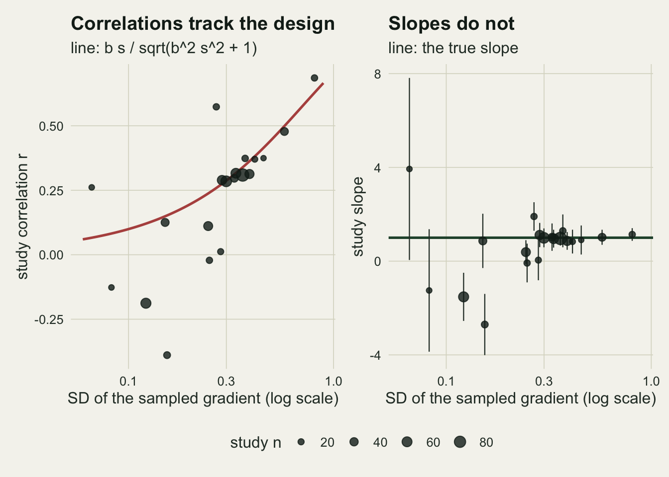
The curve is the whole mechanism. With slope b, residual standard deviation sigma and a sampled predictor standard deviation s, the population correlation of a study is b s / sqrt(b^2 s^2 + sigma^2). The correlation is the slope divided by the study’s own design. On Fisher’s scale the expression simplifies: the inverse hyperbolic tangent of u / sqrt(1 + u^2) is the inverse hyperbolic sine of u, so the expected Fisher z of a study is asinh(b s / sigma), up to the small bias of atanh(r). For a meta-analysis this gives the heterogeneity in advance: the between-study variance that the design creates is the variance of asinh(b s_i / sigma) over the twenty studies.
The spread of gradients predicts the heterogeneity
Each meta-analysis is run twice on the same studies. The correlation arm uses Fisher’s z, atanh(r), with the usual variance 1 / (n - 3). The slope arm uses the least squares slope with its standard error, which is possible here because every study measures the same variable in the same units. Both arms use DerSimonian and Laird random effects, Cochran’s Q and I-squared, and a method of moments meta-regression on log extent with a residual between-study variance and a z test, the machinery of random-effects meta-analysis and meta-regression with moderators written again in a few lines.
dl_pool <- function(y, v) {
  w <- 1 / v; k <- length(y); mu_fe <- sum(w * y) / sum(w)
  Q <- sum(w * (y - mu_fe)^2)
  t2 <- max(0, (Q - (k - 1)) / (sum(w) - sum(w^2) / sum(w)))
  ws <- 1 / (v + t2)
  c(mu = sum(ws * y) / sum(ws), pQ = pchisq(Q, k - 1, lower.tail = FALSE),
    I2 = max(0, (Q - (k - 1)) / Q), t2 = t2)
}
mm_reg <- function(y, v, X) {       # p value of the first moderator
  X <- cbind(1, X); k <- length(y); p <- ncol(X); w <- 1 / v
  XtW <- t(X * w); A <- solve(XtW %*% X)
  e <- y - X %*% (A %*% (XtW %*% y))
  QE <- sum(w * e^2)
  trP <- sum(w) - sum(diag(A %*% (t(X * w^2) %*% X)))
  t2 <- max(0, (QE - (k - p)) / trP)
  ws <- 1 / (v + t2); XtWs <- t(X * ws); V <- solve(XtWs %*% X)
  beta_hat <- V %*% (XtWs %*% y)
  2 * pnorm(-abs(beta_hat[2] / sqrt(V[2, 2])))
}
The same function also runs the repairs that the later sections discuss, so every arm sees the same simulated studies.
case2 <- function(r, U) U * r / sqrt(1 + r^2 * (U^2 - 1))
analyse_meta <- function(d) {
  r <- d$r; n <- d$n; zr <- atanh(r); vz <- 1 / (n - 3)
  U <- median(d$sx) / d$sx
  den <- 1 + r^2 * (U^2 - 1)
  rc <- case2(r, U); zc <- atanh(rc)
  v_delta <- (U / den^1.5)^2 * (1 - r^2)^2 / (n - 1) / (1 - rc^2)^2
  v_scale <- vz * (rc / r)^2
  se_known <- 1 / (d$sx * sqrt(n - 1))
  arms <- list(zr = list(zr, vz), sl = list(d$bh, d$se^2), cu = list(zc, vz),
               cd = list(zc, v_delta), cs = list(zc, v_scale))
  out <- numeric(0)
  for (nm in names(arms)) {
    pp <- dl_pool(arms[[nm]][[1]], arms[[nm]][[2]])
    out[paste0(nm, "_I2")] <- pp[["I2"]]
    out[paste0(nm, "_Q")]  <- pp[["pQ"]] < 0.05
    out[paste0(nm, "_mu")] <- pp[["mu"]]
    out[paste0(nm, "_E")]  <- mm_reg(arms[[nm]][[1]], arms[[nm]][[2]], d$log_ext) < 0.05
  }
  out["zsd_E"] <- mm_reg(zr, vz, cbind(d$log_ext, log(d$sx))) < 0.05
  out["zrg_E"] <- mm_reg(zr, vz, cbind(d$log_ext, log(d$x_range))) < 0.05
  out["slk_Q"] <- dl_pool(d$bh, se_known^2)[["pQ"]] < 0.05
  out["t2_design"] <- var(asinh(b_true * d$L / sqrt(12)))
  out["t2_zr"] <- dl_pool(zr, vz)[["t2"]]
  out["rmin"] <- min(r); out["rmax"] <- max(r)
  out
}
The grid is fixed in advance: spreads of 1, 2, 4 and 8 at rho = 0.7, each with and without true slope heterogeneity, plus two weaker couplings of extent to gradient length at the fourfold spread. Each cell has 2000 meta-analyses.
n_meta <- 2000
cells <- rbind(expand.grid(R = c(1, 2, 4, 8), rho = 0.7, cv = c(0, 0.2)),
               data.frame(R = 4, rho = c(0, 0.4), cv = 0))
cell_res <- lapply(seq_len(nrow(cells)), function(i) {
  set.seed(5270 + i)
  st <- sim_studies(n_meta, cells$R[i], cells$rho[i], cells$cv[i])
  vapply(split(st, st$meta), analyse_meta, numeric(27))
})
res <- cbind(cells, t(vapply(cell_res, rowMeans, numeric(27))))
res_sd <- t(vapply(cell_res, function(m) apply(m, 1, sd), numeric(27)))
mcse_max <- sqrt(0.25 / n_meta); mcse_05 <- sqrt(0.05 * 0.95 / n_meta)
cell <- function(R, rho = 0.7, cv = 0) which(res$R == R & res$rho == rho & res$cv == cv)
g <- function(metric_col, R, rho = 0.7, cv = 0) res[[metric_col]][cell(R, rho, cv)]
With 2000 meta-analyses per cell, a rejection rate near 0.05 carries a Monte Carlo standard error of 0.005, and no rate carries more than 0.011.
At the fourfold spread the correlation arm returns a mean I-squared of 0.51, its Q test rejects homogeneity in 78.0 per cent of meta-analyses, and log extent comes out as a significant moderator in 69.7 per cent. The slope arm, on exactly the same studies, returns an I-squared of 0.11 and a significant extent moderator in 4.7 per cent, which is the nominal five per cent within Monte Carlo error. The average meta-analysis spans study correlations from -0.09 to 0.71 with one true slope.
The closed form accounts for the between-study variance behind that I-squared. The between-study variance that the design creates, the variance of asinh(b s_i) over each meta-analysis, averages 0.0336 at the fourfold spread; the DerSimonian and Laird estimate from the correlations averages 0.0339. At the eightfold spread the two are 0.0955 and 0.0961. The meta-analysis is estimating the variance of the study designs, and estimating it well.
The slope arm’s Q test is not quite nominal either: it rejects in 8.2 per cent of meta-analyses at the fourfold spread. That excess has nothing to do with gradient length. It is present at a spread of 1 (9.9 per cent), and it goes away when the Q test uses the true within-study variances instead of the estimated ones (4.8 per cent at the fourfold spread). It is the route to spurious heterogeneity that meta-analysis of little-replicated experiments measures, small here because every study has at least 15 observations.
main_rows <- res[res$rho == 0.7 & res$cv == 0, ]
main_sd <- res_sd[res$rho == 0.7 & res$cv == 0, , drop = FALSE]
colnames(main_sd) <- colnames(res)[-(1:3)]
metric_lev <- c("mean I-squared", "Q test rejects", "extent moderator significant")
arm_lev <- c("Fisher z of r", "slopes")
sweep_df <- do.call(rbind, lapply(seq_along(metric_lev), function(j) {
  suf <- c("_I2", "_Q", "_E")[j]
  do.call(rbind, lapply(1:2, function(a) {
    col_nm <- paste0(c("zr", "sl")[a], suf)
    val <- main_rows[[col_nm]]
    se <- if (j == 1) main_sd[, col_nm] / sqrt(n_meta) else sqrt(val * (1 - val) / n_meta)
    data.frame(R = main_rows$R, metric = metric_lev[j], arm = arm_lev[a],
               value = val, se = se)
  }))
}))
sweep_df$metric <- factor(sweep_df$metric, levels = metric_lev)
sweep_df$arm <- factor(sweep_df$arm, levels = arm_lev)ggplot(sweep_df, aes(R, value, colour = arm)) +
geom_hline(data = data.frame(metric = factor(metric_lev[2:3], levels = metric_lev), h = 0.05),
aes(yintercept = h), colour = te_body, linetype = "dashed", linewidth = 0.5) +
geom_line(linewidth = 0.9) +
geom_errorbar(aes(ymin = value - 2 * se, ymax = value + 2 * se), width = 0.08,
linewidth = 0.4) +
geom_point(size = 2.2) +
facet_wrap(~ metric, nrow = 1) +
scale_x_log10(breaks = c(1, 2, 4, 8)) +
scale_y_continuous(limits = c(0, 1)) +
scale_colour_manual(values = c(te_rust, te_forest), name = NULL) +
labs(x = "spread of gradient lengths, P90 / P10 (log scale)", y = NULL,
title = "One slope, heterogeneity on demand",
subtitle = "dashed line: the nominal five per cent") +
theme_datasheet() + theme(legend.position = "bottom")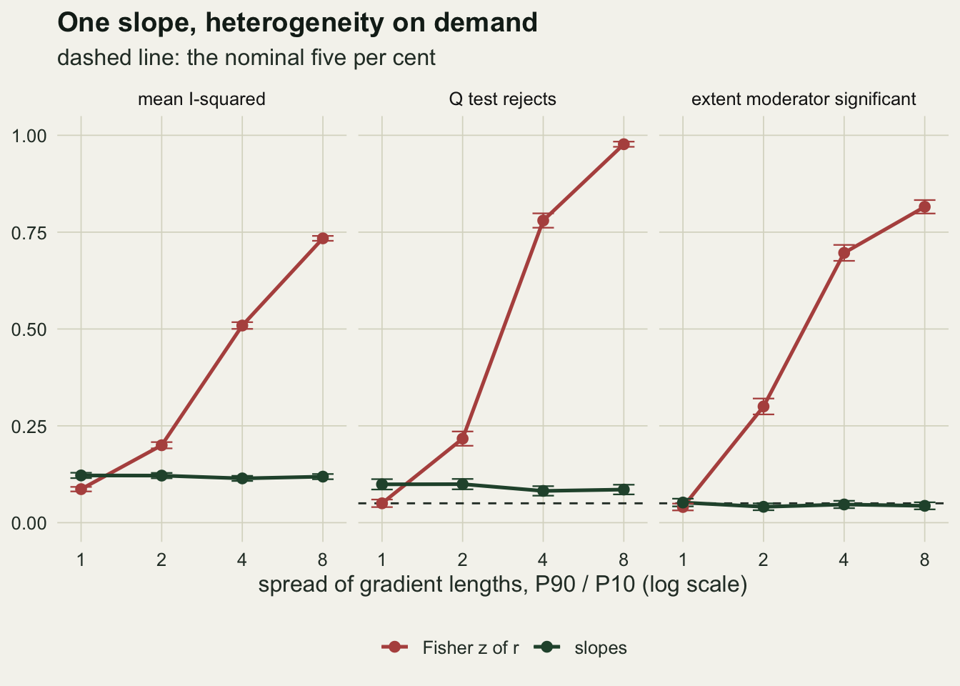
The effect grows with the spread and never stops growing inside the grid. With every study sampling the same gradient length the correlation arm is nominal: I-squared 0.09, Q rejecting in 5.0 per cent and the moderator in 4.0 per cent. At a twofold spread those become 0.20, 21.7 and 30.0 per cent; at an eightfold spread 0.73, 97.7 and 81.5 per cent. The slopes hold an I-squared between 0.11 and 0.12 and a moderator rate between 4.1 and 5.2 per cent throughout. There is no single number for this effect: it is a dose, and the dose is the spread of gradient lengths in the literature being pooled.
The pooled correlation drifts too. Back-transformed, the random-effects mean of the correlation arm is 0.304 at a spread of 1 and 0.381 at a spread of 8, while the median study’s population correlation is 0.30 in every cell. The inverse hyperbolic sine is convex on the log scale of s, so a wider spread of designs lifts the average Fisher z even though the median design has not moved.
The extent moderator is right about Zr
A significant moderator in a meta-analysis is usually read as a biological difference between the kinds of studies it separates. Here it is not, and yet the test is not miscalibrated. Fisher’s z really does differ with extent, because extent predicts gradient length and gradient length sets z. The test answers the question it was asked correctly; the question was about the correlation, and the correlation is partly a property of the design.
The coupling between extent and gradient length is what turns the design heterogeneity into a moderator, and the two extra cells vary it at the fourfold spread.
rho_rows <- res[res$R == 4 & res$cv == 0, ]
rho_rows <- rho_rows[order(rho_rows$rho), ]
rho_df <- data.frame(rho = rep(rho_rows$rho, 3),
                     arm = factor(rep(c("Fisher z of r", "slopes", "Fisher z, log SD(x) added"),
                                      each = nrow(rho_rows)),
                                  levels = c("Fisher z of r", "Fisher z, log SD(x) added", "slopes")),
                     rate = c(rho_rows$zr_E, rho_rows$sl_E, rho_rows$zsd_E))
rho_df$se <- sqrt(rho_df$rate * (1 - rho_df$rate) / n_meta)
With no coupling at all the extent moderator is significant in 6.8 per cent of meta-analyses, while the I-squared is still 0.51: the heterogeneity is all there, but extent does not track it. That rate sits a little above five per cent, the same small excess the z test shows under genuine slope heterogeneity in the section on differing slopes below. At a coupling of 0.4 the rate is 26.2 per cent and at 0.7 it is 69.7 per cent. Any study-level moderator that happens to track gradient length (region size, latitude band, the decade of the study, the kind of journal) inherits the same effect, in proportion to how closely it tracks gradient length, which is the reason this is worth knowing before a moderator table is interpreted.
ggplot(rho_df, aes(rho, rate, colour = arm)) +
  geom_hline(yintercept = 0.05, colour = te_body, linetype = "dashed", linewidth = 0.5) +
  geom_line(linewidth = 0.9) +
  geom_errorbar(aes(ymin = rate - 2 * se, ymax = rate + 2 * se), width = 0.02,
                linewidth = 0.4) +
  geom_point(size = 2.4) +
  scale_colour_manual(values = c(te_rust, te_gold, te_forest), name = NULL) +
  scale_x_continuous(breaks = c(0, 0.4, 0.7)) +
  scale_y_continuous(limits = c(0, 1)) +
  labs(x = "correlation of log extent with log gradient length",
       y = "extent moderator significant",
       title = "The moderator is only as real as the coupling",
       subtitle = "fourfold spread; dashed line: five per cent") +
  theme_datasheet() + theme(legend.position = "bottom")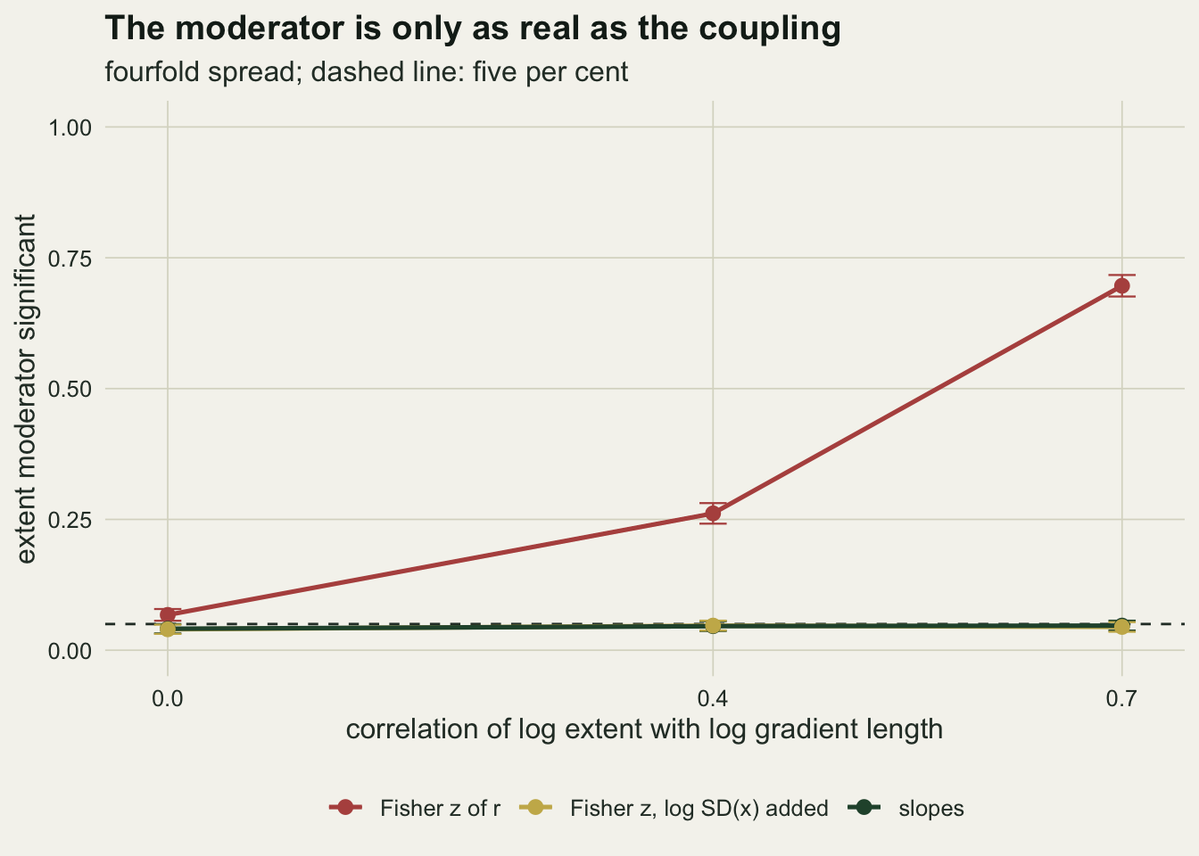
Repairs: a second moderator, or a corrected correlation
When the studies share both variables in common units the repair is the slope arm above, and nothing else is needed. When the response is measured in different units across studies (different traits, different abundance indices) but the predictor is shared, the slopes cannot be pooled, yet SD(x) is still on one scale, and a standardised effect with a known SD(x) is the common currency. Two repairs remain, and both need the standard deviation of the predictor in each study. Neither uses the units of the response, so the simulation covers this case even though its responses share one scale. When the predictors themselves differ (one study uses elevation, another temperature, a third a productivity index), their standard deviations cannot be compared, neither repair below is defined, and the design heterogeneity cannot be separated from the biology.
The first keeps Fisher’s z and adds log SD(x) as a second moderator. Extent is then tested for what it explains beyond the design. The standard deviation is not always printed, but the range of the sampled gradient usually can be read off a methods section or a figure, so the log range is run beside it as a proxy.
The second corrects each correlation to a common standard deviation before pooling, the correction for direct range restriction usually called Thorndike’s case II, which Hunter, Schmidt and Le 2006 contrast with the indirect case. Extent acts only on the range of the predictor, not on the response at a given predictor value, which is direct restriction in their terms. With U_i the ratio of the target standard deviation to study i’s own, the corrected correlation is U r / sqrt(1 + r^2 (U^2 - 1)). The target here is the median standard deviation in the meta-analysis. Under the model used here, a straight line with constant scatter, the correction is exact: substituting the population correlation for r returns b S / sqrt(b^2 S^2 + sigma^2) at the target S. The corrected correlation also has a larger sampling error, and psychometric meta-analysis has a standard first-order variance for it (Bobko and Rieck 1980). The derivative of the correction with respect to r is U / (1 + r^2 (U^2 - 1))^(3/2), so to first order the corrected correlation has variance equal to that factor squared times (1 - r^2)^2 / (n - 1), and on Fisher’s scale that is divided by (1 - r_c^2)^2. The chunk below checks the derivative numerically before it is used.
r_try <- c(-0.2, 0.1, 0.3, 0.6); U_try <- c(0.5, 1.4, 2.5, 3.5)
h_step <- 1e-6
num_deriv <- (case2(r_try + h_step, U_try) - case2(r_try - h_step, U_try)) / (2 * h_step)
ana_deriv <- U_try / (1 + r_try^2 * (U_try^2 - 1))^1.5
deriv_gap <- max(abs(num_deriv - ana_deriv))
The analytic and numerical derivatives agree to \(6.4 \times 10^{-11}\) over four combinations of r and U. Three versions of the correction are run: with the unadjusted 1 / (n - 3), which ignores what the correction does to sampling error; with this first-order (delta-method) variance; and with a cruder scaling of 1 / (n - 3) by (r_c / r)^2. None of them carries the error in each study’s own estimate of SD(x), which enters U_i.
arm_names <- c(zr = "Fisher z of r", sl = "slopes", cu = "case II, unadjusted variance",
               cd = "case II, delta-method variance", cs = "case II, variance scaled by (rc/r)^2")
rep_df <- do.call(rbind, lapply(names(arm_names), function(a)
  data.frame(R = main_rows$R, arm = arm_names[[a]],
             I2 = main_rows[[paste0(a, "_I2")]], E = main_rows[[paste0(a, "_E")]])))
rep_df <- rbind(rep_df, data.frame(R = main_rows$R, arm = "Fisher z, log SD(x) added",
                                   I2 = main_rows$zr_I2, E = main_rows$zsd_E))
rep_df$arm <- factor(rep_df$arm, levels = c(arm_names[c("zr", "cu")], "Fisher z, log SD(x) added",
                                            arm_names[c("cd", "cs", "sl")]))
rep_df$E_se <- sqrt(rep_df$E * (1 - rep_df$E) / n_meta)
Adding log SD(x) as a second moderator brings the extent test back to between 3.5 and 5.9 per cent across the four spreads, and the log range does as well, between 3.3 and 5.7 per cent. It leaves the I-squared untouched, since it is a moderator and not a new effect size: the overall heterogeneity of Fisher z is still reported, and still describes the designs.
The range correction with the unadjusted variance removes part of the problem. At the fourfold spread it leaves an I-squared of 0.28 and a moderator rate of 9.4 per cent; at the eightfold spread 0.48 and 13.1 per cent. The correction inflates the short-gradient studies by a factor U / sqrt(1 + r^2 (U^2 - 1)), which is close to U for their small correlations, and with it their sampling error, which 1 / (n - 3) does not know about, so the leftover heterogeneity is amplified noise. With the delta-method variance the same corrected correlations give an I-squared of 0.11 and a moderator rate of 3.9 per cent at the fourfold spread, and 0.13 and 4.0 per cent at the eightfold, level with the slope arm’s 0.12 and 4.3 per cent. The crude scaling gives 0.10 and 3.4 per cent at the eightfold spread. The delta-adjusted arm pools, back-transformed, to 0.305 at a spread of 1 and 0.304 at a spread of 8, against the 0.30 of the median design in every cell, because that design is the target of the correction. The range correction does not fail when it is given the variance that psychometric meta-analysis prescribes; only the unadjusted variance leaves design heterogeneity behind.
rep_long <- rbind(
  data.frame(R = rep_df$R, arm = rep_df$arm, panel = "mean I-squared",
             value = rep_df$I2, se = 0),
  data.frame(R = rep_df$R, arm = rep_df$arm, panel = "extent moderator significant",
             value = rep_df$E, se = rep_df$E_se))
rep_long <- rep_long[!(rep_long$panel == "mean I-squared" &
                       rep_long$arm == "Fisher z, log SD(x) added"), ]
rep_long$panel <- factor(rep_long$panel,
                         levels = c("mean I-squared", "extent moderator significant"))
te_amber <- "#b5651d"   # one extra hue, for the unadjusted correction only
ggplot(rep_long, aes(R, value, colour = arm, linetype = arm, shape = arm)) +
  geom_hline(data = data.frame(panel = factor("extent moderator significant",
                                              levels = levels(rep_long$panel)), h = 0.05),
             aes(yintercept = h), colour = te_body, linetype = "dashed", linewidth = 0.4) +
  geom_line(linewidth = 0.8) +
  geom_errorbar(aes(ymin = value - 2 * se, ymax = value + 2 * se), width = 0.06,
                linewidth = 0.4, linetype = "solid") +
  geom_point(size = 2.3) +
  facet_wrap(~ panel, nrow = 1) +
  scale_x_log10(breaks = c(1, 2, 4, 8)) +
  scale_y_continuous(limits = c(0, 0.85)) +
  scale_colour_manual(values = c(te_rust, te_amber, te_gold, te_ink, te_ink, te_forest),
                      name = NULL) +
  scale_linetype_manual(values = c("solid", "solid", "dashed", "solid", "dotted", "solid"),
                        name = NULL) +
  scale_shape_manual(values = c(16, 17, 1, 15, 0, 18), name = NULL) +
  guides(colour = guide_legend(ncol = 2), linetype = guide_legend(ncol = 2),
         shape = guide_legend(ncol = 2)) +
  labs(x = "spread of gradient lengths, P90 / P10 (log scale)", y = NULL,
       title = "What each repair leaves behind",
       subtitle = "dashed line: five per cent") +
  theme_datasheet() +
  theme(legend.position = "bottom", legend.key.width = unit(1.6, "lines"))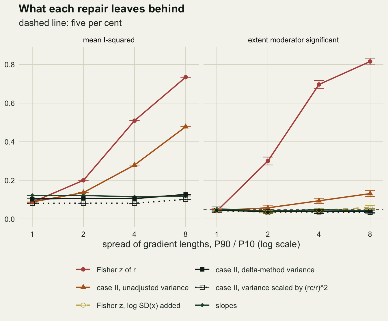
The Q test is where the corrected correlations are least tidy. With the delta-method variance it rejects homogeneity in 7.3 per cent of meta-analyses at the fourfold spread and 11.5 per cent at the eightfold, where the slopes reject in 8.6 per cent; the crude scaling gives 4.6 and 8.1 per cent. This post does not isolate the cause of the excess at the eightfold spread. Two candidates are that the delta method is a first-order approximation applied where U can reach three or more, and that the variance uses the study’s own r, so the weights are not independent of the estimates. The excess does not reach the moderator test, which is the test a reader is most likely to act on.
When the slopes really differ
Everything so far has one true slope, which is the cleanest case and not a realistic one. The second half of the grid gives each study its own slope, lognormal around 1 with a coefficient of variation of 0.2, drawn independently of extent.
The ranking does not change. At the fourfold spread the correlation arm gives an I-squared of 0.55 and a moderator rate of 62.8 per cent; the slopes give 0.23 and 6.2 per cent; Fisher z with log SD(x) added gives 5.1 per cent and the delta-adjusted correction 5.2 per cent. The slope arm’s I-squared now reflects real heterogeneity and should. Its moderator test, though, runs above five per cent once that heterogeneity is present: between 5.5 and 6.2 per cent up to the fourfold spread, and 8.6 per cent at the eightfold. The excess up to the fourfold spread is present at a spread of 1 (6.2 per cent), where every gradient has the same length, so it does not come from gradient length; the likeliest source is the z test itself, which treats the estimated between-study variance as known. At the eightfold spread the repaired correlation arms drift with it, to 7.1 per cent with log SD(x) added and 7.0 per cent for the delta-adjusted correction. A longer gradient makes a study’s slope more precise, and with extent coupled to gradient length the study weights line up with the moderator; that is a plausible route for the rise at the eightfold spread, but this post does not isolate it. The drift is small next to the 79.2 per cent of the unrepaired correlations.
What to report
Report the per-unit slope whenever the studies share the predictor and the response, each in common units, and pool slopes. It is the only effect size here that does not carry the design, and it is what the biology is about.
When a correlation or another standardised effect is unavoidable, extract the standard deviation of the predictor from every study, or failing that the sampled range, and report its spread across studies as the ratio of the 90th to the 10th percentile. That single number says how much heterogeneity the design can have made: at a spread near 1 there is nothing to worry about, and at a fourfold spread the design alone gave an I-squared of 0.51 here, against 0.11 for the same studies as slopes.
Test moderators with log SD(x) in the model. A moderator that survives it explains something beyond the design, and one that does not may still be a real moderator of the correlation, but it says nothing about how the response changes per unit of the predictor.
If the correlations are range-corrected, give the target standard deviation and use a sampling variance that carries the correction. The corrected correlation analysed with 1 / (n - 3) leaves a large part of the design heterogeneity in place, and a reader cannot tell that from the output.
Honest limits
The model is the case where the range correction is exact: a straight line with constant scatter and a predictor chosen by the study. Curved responses, residual scatter that changes along the gradient, or selection of sites on a third variable correlated with the predictor and the response (indirect restriction, in the terms of Hunter, Schmidt and Le 2006) all break the correction, and the log SD(x) moderator then removes a linear trend in the design effect and not the whole of it.
The spread of gradient lengths in real syntheses was not measured for this post. The sweep from 1 to 8 is a design choice, and fourfold is used as the centre because it is a plausible contrast between a reserve and a mountain range, not because any published synthesis was checked. The numbers here should be read against the spread in the literature at hand, which the second paragraph of the previous section tells you how to compute.
Every study reports its standard deviation correctly here. In practice SD(x) is often missing, and a range read from a figure is a noisy proxy whose error behaves like the recovery errors in effect sizes from incomplete reports. The range stood in well here because the simulated predictor is uniform; for a predictor bunched in the middle, the sampled range grows with sample size far more than it does for a uniform one, and the log range moderator then also carries log n. Neither repair carries the error of a range read from a figure, and the delta-method variance does not carry the error in each study’s own SD(x) even when it is reported.
The meta-analysis machinery is DerSimonian and Laird with a z test throughout, chosen because it is the common default and the estimator that random-effects meta-analysis introduces first. REML estimation of the between-study variance and the Knapp and Hartung adjustment of the moderator test were not run, so the small drift of the moderator test under genuine slope heterogeneity is reported for this machinery only.
Finally, twenty studies of 15 to 100 observations are one realistic size. Larger syntheses and larger studies raise the power of every test, so the same spread should produce more significant moderators, not fewer; only the twenty-study size was run. Baguley 2009 gives the general case for simple, unstandardised effects where the units allow it. Nakagawa and Cuthill 2007, who recommend d and r because meta-analysis needs them, add that unstandardised effects such as a regression coefficient are no less important. That is the same advice reached from a different direction.
References
Greenland S, Schlesselman JJ, Criqui MH 1986 American Journal of Epidemiology 123(2):203-208 (10.1093/oxfordjournals.aje.a114229)
Bobko P, Rieck A 1980 Applied Psychological Measurement 4(3):385-398 (10.1177/014662168000400309)
Hunter JE, Schmidt FL, Le H 2006 Journal of Applied Psychology 91(3):594-612 (10.1037/0021-9010.91.3.594)
DerSimonian R, Laird N 1986 Controlled Clinical Trials 7(3):177-188 (10.1016/0197-2456(86)90046-2)
Baguley T 2009 British Journal of Psychology 100(3):603-617 (10.1348/000712608X377117)
Nakagawa S, Cuthill IC 2007 Biological Reviews 82(4):591-605 (10.1111/j.1469-185X.2007.00027.x)