Coarse climate layers and a species’ niche width

Plots read from a coarse climate grid carry Berkson error and the fitted niche widens. Why a pooled correction fails on rugged cells, and a per-cell fix in R.

A vegetation survey has two thousand plots, each with a GPS position and a presence or absence of a montane grass. The temperature for each plot comes from a gridded climate product, because nobody logged temperature at two thousand plots, and the grid cell is a few kilometres across while the plot is a few metres. Every plot inside a cell receives the same value: the cell mean. A logistic regression on temperature and its square then gives the species a thermal optimum and a tolerance, and the tolerance comes out wider than the grass really is.

The reason is not noise in the climate product. The plot’s true temperature is the cell mean plus a local deviation, from a north-facing slope, a hollow that collects cold air or a ridge. The recorded value is fixed and the truth scatters around it, which is the kind of error Berkson (1950) separated from the classical error of a noisy instrument. The mechanism by which Berkson error flattens a sigmoid is already set out on this site in Checking a dose-response analysis, where the nominal concentration is fixed and the real exposure in each vessel scatters around it: the fitted curve is an average of curves centred at different places, and an average of sigmoids is a shallower sigmoid. That argument is not repeated here. This post applies it to a niche fitted on a coarse climate layer and follows it to the point where the obvious corrections stop working.

It is also not the error treated in Measurement error and regression dilution, which is classical error and its reliability-ratio correction; that correction is measured below and is wrong here. Checking a remote sensing covariate coarsens an NDVI layer under a log-linear abundance model and finds the coefficient per unit rising while the effect per standard deviation falls; there is no niche and no Berkson correction in it. MaxEnt as a Poisson point process measures how the cell-centre covariate of a count grid departs from the point-process likelihood as cells grow, which is the same misalignment seen from the likelihood side, without a niche width or a fix.

The problem has a name and a recent treatment. Mourguiart and colleagues (2024) call it area-to-point misalignment, compare a plain GLM, a spatial GLM and a Berkson error model (a model that uses the fine-grain variation within each coarse cell, as the per-cell fit below does) on virtual species across different degrees of spatial heterogeneity, and report that only the Berkson model recovers the species-environment relationship from environmental data up to fifty times coarser than the response, while both GLMs return a flattened one. The post reproduces the flattening, derives its size in the simplest case, and then measures what happens to the corrections when the within-cell variation is not the same in every cell, which is the normal state of a landscape with both plains and hills in it.

library(ggplot2)

te_paper  <- "#f5f4ee"
te_ink    <- "#16241d"
te_body   <- "#2c3a31"
te_forest <- "#275139"
te_rust   <- "#b5534e"
te_gold   <- "#c9b458"
te_line   <- "#dad9ca"

theme_datasheet <- function() {
  theme_minimal(base_size = 12) +
    theme(plot.background  = element_rect(fill = te_paper, colour = NA),
          panel.background = element_rect(fill = te_paper, colour = NA),
          panel.grid.major = element_line(colour = te_line, linewidth = 0.3),
          panel.grid.minor = element_blank(),
          text             = element_text(colour = te_body),
          plot.title       = element_text(colour = te_ink, face = "bold"),
          plot.subtitle    = element_text(colour = te_body),
          axis.text        = element_text(colour = te_body),
          strip.text       = element_text(colour = te_ink))
}

A fine landscape and three kinds of coarse cell

The landscape is a 200 by 200 grid of fine cells, standing in for the plot scale. Temperature, in standardised units, is a west to east gradient plus a smooth local texture. The texture is the within-cell variation that a coarse layer loses, and its amplitude is where the three constructions differ. In the uniform landscape the amplitude is the same everywhere, so every coarse cell has nearly the same within-cell standard deviation. In the patchy landscape the amplitude follows a second, broad random field that has nothing to do with the gradient: rugged patches next to flat ones, in no relation to how warm the cell is. In the mid-slope landscape the amplitude peaks in the middle of the gradient, a ridge running north to south. All three are scaled to the same mean squared amplitude, so the average within-cell variance is matched and only its distribution between cells changes.

The species has a Gaussian niche on the logit scale with optimum 0.3, tolerance 0.5 and a peak probability of one half, and two thousand plots are placed at random fine cells. The coarse layer is the block mean over f by f fine cells, for f of 5, 10, 20 and 40, and the within-cell standard deviation s of each block is kept as well, because that is what a finer layer can supply.

n_side   <- 200
opt_true <- 0.3
tol_true <- 0.5
lp_true  <- 0
grad_sd  <- 0.7
fine_sd  <- 0.75
rough    <- 0.8
f_set    <- c(5, 10, 20, 40)
n_plot   <- 2000
kinds    <- c("uniform", "patchy", "midslope")

expit <- function(z) 1 / (1 + exp(-z))

smooth_field <- function(n, r) {
  w_mat <- matrix(rnorm(n * n), n, n)
  d_wrap <- pmin(0:(n - 1), n - 0:(n - 1))
  k_one <- exp(-d_wrap^2 / (2 * r^2))
  z_mat <- Re(fft(fft(w_mat) * fft(outer(k_one, k_one)), inverse = TRUE))
  (z_mat - mean(z_mat)) / sd(as.vector(z_mat))
}

make_land <- function(kind, g_sd = grad_sd) {
  col_pos  <- (seq_len(n_side) - 0.5) / n_side
  gradient <- matrix(g_sd * sqrt(3) * (2 * col_pos - 1), n_side, n_side, byrow = TRUE)
  g_std    <- gradient / sd(as.vector(gradient))
  driver <- switch(kind,
    uniform  = matrix(0, n_side, n_side),
    patchy   = smooth_field(n_side, 30),
    midslope = { q_mat <- -g_std^2; (q_mat - mean(q_mat)) / sd(as.vector(q_mat)) })
  amp <- exp(rough * driver)
  amp <- fine_sd * amp / sqrt(mean(amp^2))
  gradient + amp * smooth_field(n_side, 3)
}

cell_stats <- function(x_fine, f) {
  n_c  <- n_side %/% f
  c_id <- as.vector(((row(x_fine) - 1) %/% f) * n_c + (col(x_fine) - 1) %/% f + 1)
  xv   <- as.vector(x_fine)
  m_c  <- rowsum(xv, c_id)[, 1] / f^2
  s_c  <- sqrt(pmax(rowsum(xv^2, c_id)[, 1] / f^2 - m_c^2, 0))
  list(id = c_id, m = m_c, s = s_c, n_c = n_c)
}

set.seed(34120)
map_df <- do.call(rbind, lapply(kinds, function(k) {
  cs <- cell_stats(make_land(k), 20)
  data.frame(kind = k, row_c = (seq_along(cs$s) - 1) %/% cs$n_c + 1,
             col_c = (seq_along(cs$s) - 1) %% cs$n_c + 1, s = cs$s,
             cv = sd(cs$s) / mean(cs$s))
}))
map_cv <- tapply(map_df$cv, map_df$kind, mean)
map_df$panel <- factor(map_df$kind, kinds,
  c("uniform: one texture everywhere", "patchy: rugged patches",
    "mid-slope: rugged ridge"))

ggplot(map_df, aes(col_c, row_c, fill = s)) +
  geom_tile(colour = te_paper, linewidth = 0.4) +
  facet_wrap(~ panel) +
  scale_fill_gradient(low = te_line, high = te_forest, name = "within-cell SD") +
  scale_x_continuous(breaks = c(1, 10), labels = c("cold", "warm")) +
  scale_y_continuous(breaks = NULL) +
  coord_equal() +
  labs(x = "coarse cell, west to east along the gradient", y = NULL,
       title = "The same average roughness, spread three ways") +
  theme_datasheet() +
  theme(legend.position = "bottom", panel.grid.major = element_blank())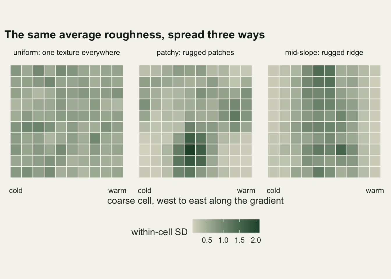

Figure 1: Within-cell standard deviation of temperature for one example of each kind, on the grid with 20 by 20 fine cells per coarse cell. All three are built with the same average within-cell variance.

The coefficient of variation of s between coarse cells, CV(s), is 0.24 for the uniform landscape in the figure, 0.70 for the patchy one and 0.63 for the mid-slope one. The uniform value is not zero because each coarse cell holds a finite piece of the texture, and that piece varies.

One within-cell SD everywhere: the widening has a closed form

When every coarse cell has the same within-cell standard deviation s and the within-cell deviations are normal, the widening can be written down. For a rare species the logit is close to the log, so the probability at a point is close to exp(lp - (x - opt)^2 / (2 tol^2)). A plot in a cell with mean m has x = m + s z with z standard normal, and the average of that Gaussian curve over z is another Gaussian in m, with the same centre, a lower peak and variance tol^2 + s^2. The fitted tolerance on the cell mean is therefore sqrt(tol^2 + s^2) and the optimum does not move. This is the standard convolution of two Gaussians, a Berkson-error result of the kind treated by Carroll and colleagues (2006); the chunk below checks it at population level, fitting every one of the 40 000 fine cells with its expected probability as the response so that no sampling noise enters, over four uniform landscapes for each of three gradient strengths.

set.seed(34104)
cf_rows <- list()
for (g_sd in c(0.35, 0.7, 1.4)) for (r in 1:4) {
  x_fine <- make_land("uniform", g_sd = g_sd)
  for (f in f_set) {
    cs  <- cell_stats(x_fine, f)
    m   <- cs$m[cs$id]
    s2  <- mean(cs$s^2)
    stopifnot(abs(mean((x_fine - mean(x_fine))^2) - mean((cs$m - mean(cs$m))^2) - s2) < 1e-8)
    lam <- (var(cs$m) - s2) / var(cs$m)
    for (lp in c(-4, 0)) {
      p_fine <- as.vector(expit(lp - (x_fine - opt_true)^2 / (2 * tol_true^2)))
      b <- unname(coef(suppressWarnings(glm(p_fine ~ m + I(m^2), family = quasibinomial))))
      cf_rows[[length(cf_rows) + 1]] <- data.frame(g_sd, lp, f,
        tol_pop = sqrt(-1 / (2 * b[3])), opt_pop = -b[2] / (2 * b[3]),
        berkson = sqrt(tol_true^2 + s2), lam = lam,
        classical = if (lam > 0) tol_true / lam else NA)
    }
  }
}
cf_all <- do.call(rbind, cf_rows)
cf_tab <- aggregate(cbind(tol_pop, opt_pop, berkson) ~ g_sd + lp + f, cf_all, mean)
cf_tab$err_berk  <- cf_tab$berkson / cf_tab$tol_pop - 1
cf_design_rare <- range(cf_tab$err_berk[cf_tab$g_sd == 0.7 & cf_tab$lp == -4])
cf_design_peak <- range(cf_tab$err_berk[cf_tab$g_sd == 0.7 & cf_tab$lp == 0])
cf_rare_all    <- range(cf_tab$err_berk[cf_tab$lp == -4])
cf_opt_range   <- range(cf_tab$opt_pop[cf_tab$g_sd == 0.7])
cf_worst       <- cf_tab[cf_tab$lp == -4, ][which.max(cf_tab$err_berk[cf_tab$lp == -4]), ]

cf_one     <- cf_all[cf_all$lp == 0, ]
cf_lam_neg <- sum(cf_one$lam <= 0)
stopifnot(all(cf_one$g_sd[cf_one$lam <= 0] < 1.4), all(cf_one$f[cf_one$lam <= 0] >= 20))
cf_class_all <- range(cf_all$classical / cf_all$tol_pop, na.rm = TRUE)

At the design gradient the formula matches the population-level fit for a rare species, peak probability expit(-4), to within 0.7 per cent at every grain. For the species used in the rest of the post, with a peak probability of one half, the log approximation is poorer and the formula overstates the fitted tolerance by 2.5 to 6.3 per cent. Across all three gradient strengths the rare-species error runs from -0.7 to +8.8 per cent, the worst case being the gentlest gradient, a gradient SD of 0.35, at f = 40, where the coarse means sample only a narrow band of temperature. The population-level optimum at the design gradient lies between 0.296 and 0.314, against a true 0.3. This reproduces the Berkson widening by simulation; it is not a new result.

The classical recipe does not transfer. The regression-dilution post estimates the reliability from the recorded values as lambda = (var(w) - var_u) / var(w) and divides by it; here the recorded value is m and the error variance is s^2, so lambda = (var(m) - s^2) / var(m), and the tolerance would be stretched by one over lambda. Under Berkson error the recorded value varies less than the truth, not more: the variance of the fine values is the variance of the cell means plus the mean of s^2, exactly (the stopifnot line checks it), so subtracting s^2 from var(m) removes variance that was never added. In 11 of the 48 landscape and grain combinations, all at the two gentler gradients and at f = 20 or 40, the estimated reliability is zero or negative and there is nothing to divide by. Where it is positive, the stretched tolerance is 0.76 to 27.1 times the population-level one, the largest where the reliability is just above zero. Under Berkson error the spread of the cell means is not what dilutes anything; only s enters.

Fitting the plots: naive, pooled, inverted and per cell

Four estimates of the tolerance are compared on every landscape. The naive fit is the logistic regression on m and m squared. The hand inverse takes the naive tolerance and removes the widening, sqrt(tol_naive^2 - s_rms^2), with s_rms the root mean square of s over cells. The two Berkson fits maximise the likelihood P(y = 1 | m, s) = E_z expit(eta(m + s z)), which averages the niche over the within-cell distribution; the pooled version gives every plot the same s_rms, and the per-cell version gives each plot the s of its own cell. The expectation is a Gauss-Hermite sum with sixteen nodes, obtained from the eigenvalues of a small tridiagonal matrix as in Golub and Welsch (1969), and the likelihood carries its analytic gradient so that each fit takes a fraction of a second.

gh_nodes <- function(k_n) {
  i_s <- seq_len(k_n - 1); jac <- matrix(0, k_n, k_n)
  jac[cbind(i_s, i_s + 1)] <- jac[cbind(i_s + 1, i_s)] <- sqrt(i_s)
  ev <- eigen(jac, symmetric = TRUE)
  list(z = ev$values, w = ev$vectors[1, ]^2)
}
gh <- gh_nodes(16)
stopifnot(abs(sum(gh$w) - 1) < 1e-10, abs(sum(gh$w * gh$z^2) - 1) < 1e-10,
          abs(sum(gh$w * gh$z^4) - 3) < 1e-8)

berk_nll <- function(th, y, m, s, nodes = gh) {
  x_q  <- m + outer(s, nodes$z)
  tl2  <- exp(2 * th[3])
  dx   <- x_q - th[2]
  p_q  <- expit(th[1] - dx^2 / (2 * tl2))
  pr   <- pmin(pmax(as.vector(p_q %*% nodes$w), 1e-12), 1 - 1e-12)
  nll  <- -sum(y * log(pr) + (1 - y) * log(1 - pr))
  a_i  <- -(y / pr - (1 - y) / (1 - pr))
  dp   <- p_q * (1 - p_q)
  attr(nll, "gradient") <- c(sum(a_i * (dp %*% nodes$w)),
                             sum(a_i * ((dp * dx / tl2) %*% nodes$w)),
                             sum(a_i * ((dp * dx^2 / tl2) %*% nodes$w)))
  nll
}

fit_berk <- function(y, m, s, start = c(lp_true, opt_true, log(tol_true)), nodes = gh) {
  o <- optim(start, function(th) as.numeric(berk_nll(th, y, m, s, nodes)),
             function(th) attr(berk_nll(th, y, m, s, nodes), "gradient"),
             method = "BFGS", control = list(maxit = 300))
  c(tol = exp(o$par[3]), opt = o$par[2], nll = o$value, conv = o$convergence)
}

fit_naive <- function(y, m) {
  g_fit <- suppressWarnings(glm(y ~ m + I(m^2), family = binomial))
  b <- unname(coef(g_fit))
  c(tol = if (b[3] < 0) sqrt(-1 / (2 * b[3])) else NA,
    opt = if (b[3] < 0) -b[2] / (2 * b[3]) else NA,
    nll = -as.numeric(logLik(g_fit)))
}

one_land <- function(kind, n_pl = n_plot) {
  x_fine <- make_land(kind)
  p_fine <- expit(lp_true - (x_fine - opt_true)^2 / (2 * tol_true^2))
  site <- sample.int(n_side^2, n_pl, replace = TRUE)
  y <- rbinom(n_pl, 1, p_fine[site])
  do.call(rbind, lapply(f_set, function(f) {
    cs <- cell_stats(x_fine, f)
    m <- cs$m[cs$id[site]]
    s <- cs$s[cs$id[site]]
    s_rms <- sqrt(mean(cs$s^2))
    nv <- fit_naive(y, m)
    bc <- fit_berk(y, m, s)
    bp <- fit_berk(y, m, rep(s_rms, n_pl))
    data.frame(kind, f, s_rms, s_max = max(cs$s), cv_s = sd(cs$s) / mean(cs$s),
      cor_ms = cor(cs$m, cs$s),
      formula = sqrt(tol_true^2 + s_rms^2),
      tol_naive = nv[["tol"]], opt_naive = nv[["opt"]],
      tol_inv = if (!is.na(nv[["tol"]]) && nv[["tol"]] > s_rms)
                  sqrt(nv[["tol"]]^2 - s_rms^2) else 0,
      tol_pool = bp[["tol"]], opt_pool = bp[["opt"]],
      tol_cell = bc[["tol"]], opt_cell = bc[["opt"]],
      d_nll = nv[["nll"]] - bc[["nll"]], conv = bc[["conv"]] + bp[["conv"]])
  }))
}

The stopifnot line checks that the nodes and weights integrate one, z squared and z to the fourth exactly against a standard normal. Every landscape below is a fresh draw: a new texture, a new ruggedness field and new plots.

n_land <- 40
set.seed(34101)
mc_res <- do.call(rbind, lapply(kinds, function(k)
  do.call(rbind, lapply(seq_len(n_land), function(r) cbind(rep = r, one_land(k))))))
stopifnot(all(mc_res$conv == 0), !anyNA(mc_res$tol_naive))

mc_res$aic_win <- mc_res$d_nll > 1
mc_cols <- c("s_rms", "cv_s", "cor_ms", "formula", "tol_naive", "opt_naive", "tol_inv",
             "tol_pool", "opt_pool", "tol_cell", "opt_cell", "aic_win")
mc_tab <- aggregate(mc_res[, mc_cols], by = list(kind = mc_res$kind, f = mc_res$f), FUN = mean)
mc_se  <- aggregate(mc_res[, mc_cols], by = list(kind = mc_res$kind, f = mc_res$f),
                    FUN = function(v) sd(v) / sqrt(length(v)))
mv <- function(k, f, v) mc_tab[mc_tab$kind == k & mc_tab$f == f, v]
se_tol_max <- max(unlist(mc_se[, c("tol_naive", "tol_pool", "tol_cell")]))
se_opt_max <- max(unlist(mc_se[, c("opt_naive", "opt_pool", "opt_cell")]))
cell_range <- range(mc_tab$tol_cell)
cellopt_range <- range(mc_tab$opt_cell)

Over 40 landscapes of each kind the Monte Carlo standard error of a mean tolerance is at most 0.026 and of a mean optimum at most 0.018.

On the uniform landscapes the naive tolerance behaves as the closed form says, a little below it as the peak-probability check above predicted: 0.581 against a formula value of 0.596 at f = 5, and 0.832 against 0.893 at f = 40. The naive optimum stays between 0.293 and 0.301. The pooled Berkson fit returns 0.490 at f = 20 and 0.492 at f = 40, within 0.012 of the true 0.5 at every grain. The hand inverse does not: because the formula overstates the widening at this peak probability, subtracting it removes too much, and the inverse falls to 0.396 at f = 20 and 0.351 at f = 40, 21 and 30 per cent short of the truth. With one s everywhere the pooled likelihood is enough, and the formula is a fair guide only for a rare species.

When s differs between cells, only the per-cell fit works

The patchy landscape has the same average within-cell variance, and the correlation between cell mean and cell SD averages 0.016 at f = 20: the rugged patches are no warmer or colder than the flat ones. Nothing about the gradient has changed. The corrections fail anyway.

pat <- mc_tab[mc_tab$kind == "patchy", ]
mid <- mc_tab[mc_tab$kind == "midslope", ]
pat_formula_over <- pat$formula / pat$tol_naive - 1
aic_patchy <- mc_tab$aic_win[mc_tab$kind == "patchy"]

set.seed(34105)
small_res <- do.call(rbind, lapply(seq_len(n_land), function(r) one_land("patchy", n_pl = 500)))
small_res$aic_win <- small_res$d_nll > 1
small_tab <- aggregate(small_res[, c("tol_pool", "tol_cell", "opt_cell", "aic_win")],
                       by = list(f = small_res$f), FUN = mean)

At f = 20 the naive tolerance on the patchy landscapes is 0.712, well below the formula’s 0.840; the formula now overstates the widening by 18 per cent at f = 20 and 26 per cent at f = 40. An average of Gaussian curves of different widths is not a Gaussian curve of the average width. By the closed form above, the curve from a flat cell is both narrower and taller than the curve from a rough one, so the average is more sharply peaked than a single Gaussian with the root mean square widening, and the widening the fit sees is smaller than s_rms implies.

Every correction that uses s_rms inherits the mistake. The pooled Berkson fit returns 0.343 at f = 20 and 0.333 at f = 40, a niche 0.69 and 0.67 times as wide as the real one: the widening it assumes is larger than the widening in the data, so it corrects too far. The hand inverse, which subtracts the same overstated widening from a naive tolerance that never reached it, collapses to 0.196 and 0.084. The per-cell Berkson fit, given each plot’s own s from the fine layer (in this setting, the kind of model Mourguiart and colleagues call a Berkson error model), returns 0.500 and 0.497, with an optimum of 0.295 and 0.297. Across all three landscape kinds and all four grains its mean tolerance lies between 0.492 and 0.506 and its mean optimum between 0.287 and 0.304.

The per-cell fit is also the one AIC prefers. Both fits have three parameters, so AIC compares likelihoods directly; the per-cell Berkson fit beats the naive one by more than two AIC units in 98 to 100 per cent of patchy landscapes across the four grains at two thousand plots. On the uniform landscapes the share is only 42 per cent at f = 40, although the naive tolerance there is 0.832: when AIC does not prefer the per-cell fit, the naive niche width can still be wrong. With five hundred plots the share is 80 to 95 per cent, and the per-cell tolerance is still 0.490 to 0.509 while the pooled one is 0.364 at f = 20: the failure does not go away with smaller samples. Mourguiart and colleagues make a different point about selection: because their predictions are made from the coarse covariate, the Berkson model predicts worse than the two GLMs, so selection on predictive performance would not pick it. The AIC here compares in-sample likelihoods with each plot’s own s supplied, which is a different comparison: a good fit to the plots is not the same as good prediction from the coarse layer.

The optimum moves as well, and the pooled fix misses it

The mid-slope landscape puts the rugged cells in the middle of the gradient. The correlation between cell mean and cell SD is again near zero, -0.007 at f = 20, because the dependence is not linear: roughness rises and then falls along the gradient.

Here the pooled fit fails in a different way. Its tolerance is 0.384 at f = 20 and 0.433 at f = 40, closer to the truth than on the patchy landscapes, but its optimum has moved to 0.397 and 0.490, following the naive optimum of 0.385 and 0.484. A single s removes the same widening everywhere, so it narrows the curve but does not bring its peak back. How far and which way the naive optimum moves depends on where the rough cells sit relative to the niche and to the sampled range of the gradient; this post measures one arrangement and does not map the others. The per-cell fit returns an optimum of 0.302 and 0.302 and a tolerance of 0.500 and 0.492.

On the patchy landscapes, by contrast, the optimum moves much less: the naive value is 0.329 at f = 20 and the pooled 0.324. So the pooled s fails in two distinct ways: it over-corrects the tolerance on both kinds, pushing it below the truth, most on the patchy ones, and on the mid-slope ones it also leaves the optimum displaced. The two constructions differ in where the rough cells are and, somewhat, in how unequal they are (CV(s) at f = 20 averages 0.79 on the patchy landscapes and 0.63 on the mid-slope ones), so which failure a real layer produces cannot be guessed without looking at its s.

plot_cols <- data.frame(
  col    = c("tol_naive", "tol_inv", "tol_pool", "tol_cell", "opt_naive", "opt_pool", "opt_cell"),
  qty    = rep(c("tolerance", "optimum"), c(4, 3)),
  method = c("naive", "hand inverse", "pooled s", "per-cell s", "naive", "pooled s", "per-cell s"))
long_tab <- do.call(rbind, lapply(seq_len(nrow(plot_cols)), function(i)
  data.frame(mc_tab[, c("kind", "f")], qty = plot_cols$qty[i],
             method = plot_cols$method[i], val = mc_tab[[plot_cols$col[i]]])))
long_tab$qty    <- factor(long_tab$qty, c("tolerance", "optimum"))
long_tab$kind   <- factor(long_tab$kind, kinds, c("uniform", "patchy", "mid-slope"))
long_tab$method <- factor(long_tab$method, c("naive", "hand inverse", "pooled s", "per-cell s"))
truth_df <- data.frame(qty = factor(c("tolerance", "optimum"), c("tolerance", "optimum")),
                       val = c(tol_true, opt_true))

ggplot(long_tab, aes(f, val, colour = method)) +
  geom_hline(data = truth_df, aes(yintercept = val), linetype = "dashed",
             colour = te_body, linewidth = 0.5, show.legend = FALSE) +
  geom_line(linewidth = 0.9) +
  geom_point(size = 2.2) +
  facet_grid(qty ~ kind, scales = "free_y") +
  scale_x_log10(breaks = f_set) +
  scale_colour_manual(values = c(te_rust, te_ink, te_gold, te_forest), name = NULL) +
  labs(x = "fine cells per coarse cell side (log scale)", y = NULL,
       title = "One s for every cell is not enough") +
  theme_datasheet() +
  theme(legend.position = "bottom")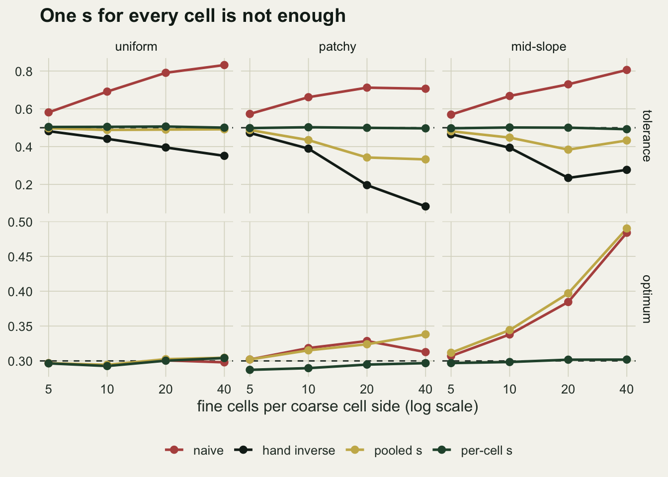

Figure 2: Mean fitted tolerance (top) and optimum (bottom) over forty landscapes of each kind, by coarse cell size. Dashed lines mark the true values.

What decides it: how much s varies between cells

The correlation between cell mean and cell SD is near zero in all three kinds of landscape, and the pooled fit works on one of them and fails on two. What separates them is how unequal the cells are, CV(s), together with how large s is against the tolerance.

diag_tab <- mc_tab[, c("kind", "f", "s_rms", "cv_s", "cor_ms", "tol_pool", "tol_cell")]
diag_tab$s_over_tol <- diag_tab$s_rms / tol_true
diag_tab$pool_gap   <- diag_tab$tol_pool - diag_tab$tol_cell
print(format(diag_tab[order(diag_tab$f, diag_tab$kind), ], digits = 3), row.names = FALSE)

     kind  f s_rms  cv_s    cor_ms tol_pool tol_cell s_over_tol pool_gap
 midslope  5 0.328 0.792  0.002138    0.481    0.497      0.655 -0.01562
   patchy  5 0.324 0.967  0.010231    0.488    0.498      0.647 -0.01002
  uniform  5 0.325 0.448  0.000739    0.497    0.504      0.650 -0.00685
 midslope 10 0.535 0.717 -0.000313    0.448    0.501      1.069 -0.05353
   patchy 10 0.531 0.889  0.015303    0.435    0.503      1.062 -0.06798
  uniform 10 0.530 0.348 -0.004043    0.488    0.505      1.060 -0.01649
 midslope 20 0.681 0.629 -0.007376    0.384    0.500      1.363 -0.11623
   patchy 20 0.675 0.787  0.015908    0.343    0.500      1.349 -0.15691
  uniform 20 0.677 0.223 -0.013508    0.490    0.506      1.354 -0.01624
 midslope 40 0.743 0.533 -0.005781    0.433    0.492      1.486 -0.05965
   patchy 40 0.736 0.655  0.023286    0.333    0.497      1.471 -0.16421
  uniform 40 0.739 0.127 -0.022663    0.492    0.500      1.479 -0.00869

mc_res$pool_gap <- mc_res$tol_pool - mc_res$tol_cell
within_cor <- sapply(c("patchy", "midslope"), function(k) sapply(f_set, function(f) {
  d_sub <- mc_res[mc_res$kind == k & mc_res$f == f, ]
  cor(d_sub$cv_s, d_sub$pool_gap)
}))
het <- mc_res[mc_res$kind != "uniform" & mc_res$f >= 10, ]
het$s_over_tol <- het$s_rms / tol_true
het$abs_cor    <- abs(het$cor_ms)
gap_lm <- coef(summary(lm(pool_gap ~ cv_s + s_over_tol + abs_cor, data = het)))
cv_uni <- range(diag_tab$cv_s[diag_tab$kind == "uniform"])
cv_het <- range(diag_tab$cv_s[diag_tab$kind != "uniform"])
cv_uni_f5 <- diag_tab$cv_s[diag_tab$kind == "uniform" & diag_tab$f == 5]
stopifnot(cv_uni_f5 == cv_uni[2], diag_tab$f[which.max(diag_tab$cv_s)] == 5,
          diag_tab$kind[which.max(diag_tab$cv_s)] == "patchy")
gap_uni <- range(diag_tab$pool_gap[diag_tab$kind == "uniform"])
dg <- function(k, f, v) diag_tab[diag_tab$kind == k & diag_tab$f == f, v]

On the uniform landscapes CV(s) is 0.13 to 0.45, the top of that range at f = 5, where each coarse cell holds only a small piece of the texture, and the pooled tolerance stays within 0.016 of the per-cell one at every grain. On the patchy and mid-slope landscapes CV(s) is 0.53 to 0.97. That alone is not enough for failure. At f = 5, where s_rms is 0.65 of the tolerance, the pooled fit on the patchy landscapes differs from the per-cell one by only -0.010, and the hand inverse returns 0.473: with s this small, every correction lands within 0.035 of the truth. At f = 10, where s_rms is 1.06 of the tolerance, the pooled gap on the patchy landscapes is -0.068 and on the mid-slope ones -0.054; at f = 20 and 40, with s_rms at 1.35 and 1.47 of the tolerance, the patchy gap is -0.157 and -0.164. As a share of the true tolerance the patchy gap is 2 per cent at f = 5, 14 per cent at f = 10 and 31 per cent at f = 20: it grows with s_rms / tol through the band from 0.65 to 1.35 rather than switching on at a threshold.

Within the patchy kind alone, where every landscape comes from the same recipe, the landscapes with more unequal cells also have the larger gap: the correlation between CV(s) and the pooled gap is -0.42 at f = 10, -0.35 at f = 20 and -0.48 at f = 40. Within the mid-slope kind the same correlation is -0.41 at f = 10 but only -0.06 and -0.17 at f = 20 and 40, so there the within-kind evidence is weak. Each landscape’s gap carries the sampling noise of two fits on two thousand plots, which is part of why all these correlations are moderate at best.

Across kinds, the split in CV(s) between the uniform and the heterogeneous landscapes is built into the design and proves nothing by itself. A linear regression of the gap on CV(s), s_rms / tol and the absolute correlation between m and s, over the 240 heterogeneous landscape and grain rows at f = 10 and coarser, gives slopes of -0.30 (standard error 0.06) for CV(s), -0.27 (0.04) for s_rms / tol and -0.07 (0.04) for the correlation. Each landscape enters at three grains, so the rows are not independent and these standard errors are too small; the reading is only that the gap goes with CV(s) and with s against the tolerance, and hardly with the correlation. Neither gives a threshold: at f = 5 the patchy landscapes have the highest CV(s) of all and almost no gap.

mc_res$kind_lab <- factor(mc_res$kind, kinds, c("uniform", "patchy", "mid-slope"))
f_lab <- sapply(f_set, function(f)
  sprintf("f = %d, mean s_rms / tol = %.2f", f, mean(diag_tab$s_over_tol[diag_tab$f == f])))
mc_res$f_lab <- factor(mc_res$f, f_set, f_lab)

ggplot(mc_res, aes(cv_s, pool_gap, colour = kind_lab)) +
  geom_hline(yintercept = 0, colour = te_body, linewidth = 0.5) +
  geom_point(size = 1.6, alpha = 0.75) +
  facet_wrap(~ f_lab, nrow = 2) +
  scale_colour_manual(values = c(te_forest, te_rust, te_gold), name = NULL) +
  labs(x = "CV(s): between-cell coefficient of variation of the within-cell SD",
       y = "pooled minus per-cell tolerance",
       title = "Unequal cells and a large s break the pooled fix") +
  theme_datasheet() +
  theme(legend.position = "bottom")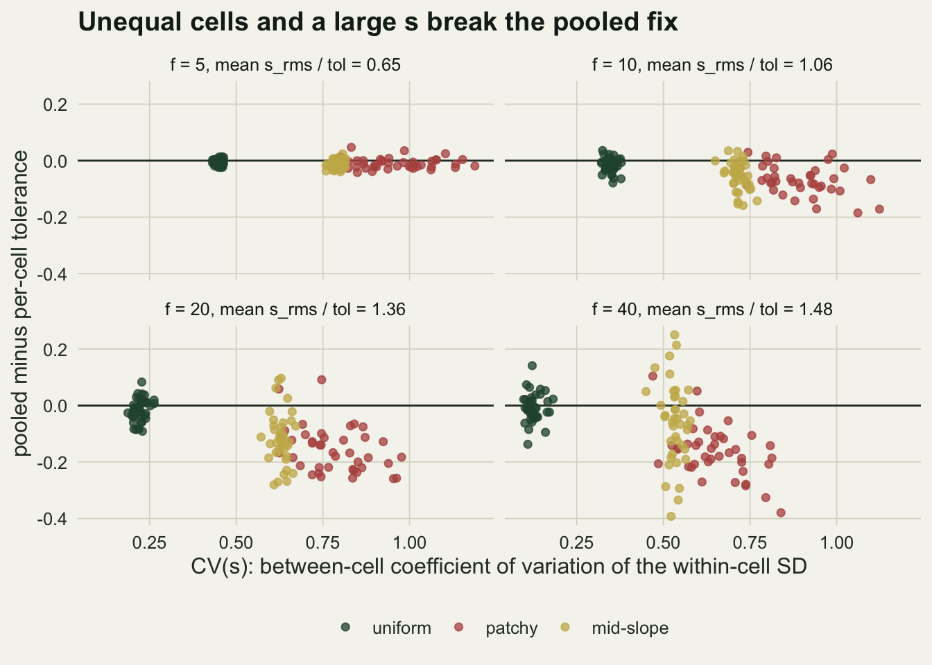

Figure 3: Pooled-s tolerance minus per-cell tolerance for each landscape against CV(s), the between-cell coefficient of variation of the within-cell SD, at each coarse grain.

The plots cannot pin down the within-cell SD

If s is what matters, it is tempting to estimate it from the survey instead of supplying it: add a fourth parameter, one s for all cells, and let the likelihood choose. On uniform landscapes, where one s is the right model, that fit is tried below with three starting values for s, keeping the best.

nll_free <- function(th, y, m) as.numeric(berk_nll(th[1:3], y, m, rep(exp(th[4]), length(m))))
set.seed(34103)
free_tab <- do.call(rbind, lapply(1:12, function(r) {
  x_fine <- make_land("uniform")
  p_fine <- expit(lp_true - (x_fine - opt_true)^2 / (2 * tol_true^2))
  site <- sample.int(n_side^2, n_plot, replace = TRUE)
  y <- rbinom(n_plot, 1, p_fine[site])
  cs <- cell_stats(x_fine, 20)
  m <- cs$m[cs$id[site]]
  nv <- fit_naive(y, m)
  best <- NULL
  for (s0 in c(0.1, 0.4, 0.8)) {
    o <- optim(c(lp_true, opt_true, log(tol_true), log(s0)), nll_free, y = y, m = m,
               method = "BFGS", control = list(maxit = 500))
    if (is.null(best) || o$value < best$value) best <- o
  }
  data.frame(s_true = sqrt(mean(cs$s^2)), s_hat = exp(best$par[4]),
             tol_hat = exp(best$par[3]), gain = nv[["nll"]] - best$value)
}))
free_s    <- range(free_tab$s_hat)
free_tol  <- range(free_tab$tol_hat)
free_true <- mean(free_tab$s_true)
free_gain <- max(free_tab$gain)
n_zero    <- sum(free_tab$s_hat < 0.05)
near      <- abs(free_tab$s_hat - free_tab$s_true) < 0.15
free_near <- range(free_tab$s_hat[near])
stopifnot(sum(near) + n_zero == nrow(free_tab))
crit_gain <- qchisq(0.90, 1) / 2
n_signif  <- sum(free_tab$gain > crit_gain)

Over 12 landscapes at f = 20, with a true s_rms of 0.68, the estimated s lands within 0.15 of the landscape’s own s_rms in 9 cases, at 0.617 to 0.798, and at essentially zero in the other 3; the tolerance that comes with it runs from 0.325 to 0.809. The largest gain in log-likelihood over the naive fit, which is the same model with s fixed at zero, is 1.27. Because s cannot be negative, the likelihood ratio test of s = 0 is judged against a half-and-half mixture of zero and a chi-squared with one degree of freedom, which at the five per cent level needs a gain of 1.35; 0 of the 12 landscapes reach it. So the estimate is often in the right place, but the plots cannot back it: in no landscape is the fit with s at its estimate detectably better than the fit with s at zero. The plots cannot tell a narrow niche seen through rough cells from a wide niche seen through smooth ones: the curve on m has a width and a height, and both are explained equally well either way. The within-cell SD has to come from outside the survey, from a finer layer.

Obscured coordinates: a second draw inside the cell

iNaturalist moves the public position of some records on purpose. Observations of a taxon whose conservation status carries an “obscured” geoprivacy setting, worldwide or in a named place, are obscured automatically, and an observer can obscure any record of their own. According to the iNaturalist help page on geoprivacy, the latitude and longitude are then replaced with a random point within a 0.2 by 0.2 degree cell, and the public positional accuracy becomes the diagonal of that cell. In the Darwin Core export that GBIF indexes (lib/darwin_core/occurrence.rb in the iNaturalist source), decimalLatitude and decimalLongitude hold the random point, coordinateUncertaintyInMeters holds that accuracy, and informationWithheld gives the reason, Coordinate uncertainty increased to <N>m to protect threatened taxon or ... at the request of the observer; the event date is exported in full. Koo and colleagues (2025) compared obscured and original iNaturalist records of three threatened species and found shifted elevational ranges and environmental values and different modelled distributions.

Take the obscuring cell to be the coarse cell of this post, give every plot, present or absent, a public point at a random fine cell of its own coarse cell, and read the temperature there. The true value is the cell mean plus one within-cell deviation, and the public value is the cell mean plus another, independent one. If the cell means were spread evenly along a long gradient, with normal within-cell deviations as above, the true value given the public value would be normal around it with variance 2 s^2, twice the Berkson error of the cell mean, and the naive tolerance would be sqrt(tol^2 + 2 s^2). The gradient here is short. The public value is the cell mean plus classical error, the kind Measurement error and regression dilution treats, and the classical recipe’s reliability ratio above, lambda = (var(w) - var_u) / var(w), is now the right quantity: with the public value as w and s^2 as var_u it equals V / (V + s^2), V being the variance of the cell means. If the cell means are also normal, with mean mu, the cell mean given the public value is pulled towards mu by the factor lambda (the regression-calibration step of Carroll and colleagues, 2006), the true value then scatters around it with variance (1 + lambda) s^2, and the curve on the public value has a tolerance of sqrt(tol^2 + (1 + lambda) s^2) / lambda and an optimum moved away from mu, to mu + (opt - mu) / lambda. At lambda = 1 this is the flat case. It is Gaussian arithmetic, and the underlying point, that positional error harms a distribution model most where the predictor changes over short distances, is made by Naimi and colleagues (2014). The chunk checks both formulas at population level for a rare species, as the closed-form check above does, on uniform landscapes at the design gradient and at twice and four times its strength.

ob_pop <- function(g_sd, f) {
  x_fine <- make_land("uniform", g_sd = g_sd)
  xv  <- as.vector(x_fine)
  cs  <- cell_stats(x_fine, f)
  s2  <- mean(cs$s^2)
  lam <- 1 - s2 / mean((xv - mean(xv))^2)                # V / (V + s^2), exactly
  p_fine <- expit(-4 - (xv - opt_true)^2 / (2 * tol_true^2))
  p_cell <- rowsum(p_fine, cs$id)[, 1] / f^2             # chance of a presence given the cell
  b <- unname(coef(suppressWarnings(glm(p_cell[cs$id] ~ xv + I(xv^2), family = quasibinomial))))
  data.frame(g_sd, f, lam, tol_pub = sqrt(-1 / (2 * b[3])), opt_pub = -b[2] / (2 * b[3]),
             flat = sqrt(tol_true^2 + 2 * s2), normal = sqrt(tol_true^2 + (1 + lam) * s2) / lam,
             opt_normal = mean(xv) + (opt_true - mean(xv)) / lam,
             kurt = mean((cs$m - mean(cs$m))^4) / mean((cs$m - mean(cs$m))^2)^2)
}
set.seed(34108)
ob_grid <- expand.grid(rep = 1:3, f = c(10, 20), g_sd = c(0.7, 1.4, 2.8))
ob_pop_tab <- aggregate(. ~ g_sd + f, do.call(rbind, Map(ob_pop, ob_grid$g_sd, ob_grid$f)), mean)
ob_pop_tab$err_flat   <- ob_pop_tab$flat / ob_pop_tab$tol_pub - 1
ob_pop_tab$err_normal <- ob_pop_tab$normal / ob_pop_tab$tol_pub - 1
print(format(ob_pop_tab, digits = 3), row.names = FALSE)

 g_sd  f   lam tol_pub opt_pub  flat normal opt_normal kurt err_flat err_normal
  0.7 10 0.726   1.144   0.446 0.900  1.180      0.414 2.51  -0.2136     0.0312
  1.4 10 0.888   0.963   0.332 0.898  0.993      0.338 2.12  -0.0673     0.0303
  2.8 10 0.964   0.908   0.292 0.922  0.950      0.311 1.85   0.0150     0.0458
  0.7 20 0.581   1.756   0.662 1.071  1.686      0.516 2.24  -0.3897    -0.0395
  1.4 20 0.806   1.300   0.400 1.102  1.314      0.372 1.86  -0.1526     0.0106
  2.8 20 0.938   1.156   0.313 1.143  1.203      0.320 1.82  -0.0112     0.0411

op <- function(g, f, v) ob_pop_tab[ob_pop_tab$g_sd == g & ob_pop_tab$f == f, v]

At the design gradient the population-level tolerance at the public point is 1.144 at f = 10 and 1.756 at f = 20, and the flat formula gives only 0.900 and 1.071, 21 and 39 per cent short. On the gradient four times as strong, where lambda is 0.96 and 0.94, the simulation reproduces the flat formula to within 1.5 per cent. The normal formula is within 4.6 per cent in all six combinations; on the strongest gradient, where the cell means are spread evenly rather than normally, the flat formula is the closer of the two, so the normal form is a guide to the size of the effect, not a correction. The optimum at the public point moves from 0.3 to 0.446 and 0.662 on the design gradient; the normal formula predicts 0.414 and 0.516, right in direction but short of the move, most at f = 20, where the cell means are furthest from a normal (kurtosis 2.24 against 2.51 at f = 10, and 3 for a normal). The shift is not a property of obscuring alone: it needs a gradient that is short against s and an optimum away from the middle of it, and on the strongest gradient the optimum stays at 0.292 and 0.313. The plots below use the species of this post, whose peak probability of one half makes the formulas only a guide, as for the cell mean above. Each landscape gets one set of plots, read four ways at f = 10 and 20.

ob_one <- function(f_obs = c(10, 20)) {
  x_fine <- make_land("uniform")
  p_fine <- expit(lp_true - (x_fine - opt_true)^2 / (2 * tol_true^2))
  site <- sample.int(n_side^2, n_plot, replace = TRUE)
  y <- rbinom(n_plot, 1, p_fine[site])
  do.call(rbind, lapply(f_obs, function(f) {
    cs <- cell_stats(x_fine, f)
    in_cell <- split(seq_len(n_side^2), cs$id)
    pub <- vapply(in_cell[cs$id[site]], function(v) v[sample.int(length(v), 1)], 1L)
    m <- cs$m[cs$id[site]]
    s <- cs$s[cs$id[site]]
    fits <- rbind(exact = fit_naive(y, x_fine[site])[1:2], public = fit_naive(y, x_fine[pub])[1:2],
                  cell_mean = fit_naive(y, m)[1:2], per_cell = fit_berk(y, m, s)[1:2])
    data.frame(f, method = rownames(fits), fits, row.names = NULL)
  }))
}
ob_n_land <- 30
set.seed(34107)
ob_res <- do.call(rbind, lapply(seq_len(ob_n_land), function(r) ob_one()))
stopifnot(!anyNA(ob_res$tol))
ob_tab <- aggregate(cbind(tol, opt) ~ method + f, ob_res, mean)
ob_se  <- aggregate(cbind(tol, opt) ~ method + f, ob_res, function(v) sd(v) / sqrt(length(v)))
ot <- function(k, f, v) ob_tab[ob_tab$method == k & ob_tab$f == f, v]

Over 30 landscapes the exact positions give a tolerance of 0.504. The public point gives 1.092 at f = 10 and 1.747 at f = 20, with the optimum at 0.429 and 0.693 (Monte Carlo standard errors up to 0.060 and 0.057); the cell mean of the same cell gives 0.695 and 0.782, and the per-cell fit 0.505 and 0.512, with the optimum at 0.290 and 0.296 (standard errors up to 0.014 for the other tolerances). The public point is worse than the cell mean at both grains, and much worse on this short gradient. Once the cell is known the public point adds nothing, so the per-cell fit is the same fit as in the sections above; it needs the cell. With obscured records, read the climate as the mean over the record’s cell, or better fit the per-cell likelihood with that cell’s s, not at the public point.

ob_side <- 0.2 * 111.32                                     # km in 0.2 degrees of latitude
ob_diag <- function(lat) sqrt(ob_side^2 + (ob_side * cos(lat * pi / 180))^2)
ob_cell <- function(coord) round(coord * 1e6) %/% 200000    # index of a fixed 0.2-degree cell
stopifnot(ob_cell(c(47.4, 47.59999, -0.1)) == c(237, 237, -1), floor(47.4 / 0.2) == 236)
round(c(side_km = ob_side, diag_km_0N = ob_diag(0), diag_km_47N = ob_diag(47), diag_km_70N = ob_diag(70)), 1)

    side_km  diag_km_0N diag_km_47N diag_km_70N 
       22.3        31.5        26.9        23.5 

The obvious recovery is floor(x / 0.2) * 0.2. That the cells sit at fixed multiples of 0.2 degrees is reported by an iNaturalist forum moderator, not documented; check it on records whose true position you know, such as your own obscured observations, before relying on it. If it holds, the cell index is an integer division done in whole micro-degrees, as in Records on grid lines and floating point in R: floor(47.4 / 0.2) returns 236 where the index is 237. The diagonal is 31 km at the equator, 27 km at 47 degrees north and 24 km at 70 degrees north, and the north to south side alone is 22 km, so an uncertainty ceiling of 10 km, the one in Cleaning GBIF and iNaturalist records in R, removes every obscured record wherever it is. That is a filter on conservation status and on observers’ choices, and neither is random in space: a status can apply in one place only, and observers decide which of their records to obscure. Coordinate error and habitat assignment measures what a filter on reported uncertainty does to a sample. For a rare species the population check above is also the presence-only case, records at public points against background points at exact positions, because the public points of plots placed at random are themselves spread evenly over the landscape, as background points are; the plots here are presence-absence.

A real elevation layer

What CV(s) and s look like on a real layer can be checked without a download. The terra package ships a small elevation raster of Luxembourg on a grid of 30 arc seconds; converting it to a temperature offset with a standard lapse rate of 6.5 degrees per kilometre, and aggregating by 3, 5 and 10 cells, gives the within-cell SD a coarse climate grid would hide.

library(terra)
elev <- rast(system.file("ex/elev.tif", package = "terra"))
temp_c <- -0.0065 * elev
dem_tab <- do.call(rbind, lapply(c(3, 5, 10), function(f) {
  m_r <- terra::aggregate(temp_c, f, mean, na.rm = TRUE)
  s_r <- terra::aggregate(temp_c, f, sd, na.rm = TRUE)
  v <- na.omit(cbind(terra::values(m_r), terra::values(s_r)))
  data.frame(f, cells = nrow(v), cor_ms = cor(v[, 1], v[, 2]),
             cv_s = sd(v[, 2]) / mean(v[, 2]), s_rms = sqrt(mean(v[, 2]^2)),
             s_q10 = unname(quantile(v[, 2], 0.1)), s_q90 = unname(quantile(v[, 2], 0.9)))
}))
print(format(dem_tab, digits = 3), row.names = FALSE)

  f cells  cor_ms  cv_s s_rms  s_q10 s_q90
  3   547 0.00911 0.575 0.172 0.0609 0.270
  5   212 0.05284 0.459 0.212 0.0913 0.308
 10    62 0.09524 0.406 0.265 0.1288 0.378

stopifnot(min(dem_tab$cv_s) < cv_uni[2], max(dem_tab$cv_s) > cv_het[1])
dem_res <- terra::res(elev)[1]
dem_lat <- mean(as.vector(terra::ext(elev))[3:4])
km_ns   <- dem_res * 111.32
km_ew   <- km_ns * cos(dem_lat * pi / 180)
tol_c <- 3
alp_sd <- c(150L, 450L)
alp_s  <- alp_sd * 0.0065

The raster’s cells are 0.00833 degrees on a side, 0.93 km north to south and 0.60 km east to west at this latitude, so the coarsest cells here are about 9 by 6 km. At aggregation factors of 3, 5 and 10 the correlation between the coarse cell mean and s is 0.01, 0.05 and 0.10, while CV(s) is 0.57, 0.46 and 0.41. These values straddle the two ranges above, the uniform landscapes at 0.13 to 0.45 and the heterogeneous ones at 0.53 to 0.97, so by themselves they settle little. The uniform landscapes show how much CV(s) a small coarse cell produces on its own: 0.45 at f = 5, where each coarse cell holds 25 fine cells, with the same texture everywhere. The coarse cells here hold at most 9, 25 and 100 raster cells, so part of their CV(s) may be of that kind. The deciding number here is s itself, and it is tiny. Its root mean square is 0.17 to 0.27 degrees, and the 10th to 90th percentiles of s over cells span from 0.06 degrees at the smallest aggregation to 0.38 at the largest. Against a thermal tolerance of 3 degrees, a round value chosen for illustration rather than taken from any species, s_rms / tol is at most 0.09, far below the f = 5 case above in which every correction worked. For a thermal niche in Luxembourg at these grains the misalignment is negligible, and the naive fit would do.

Mountains are the other end. On a 10 km climate grid over alpine terrain, a within-cell elevation standard deviation of 150 to 450 m is plausible, and by the same lapse rate that is an s of 1.0 to 2.9 degrees; the cold cells there are also likely to be the rugged ones. That is an expectation, not something measured in this post; the point of the Luxembourg numbers is that the diagnostic is cheap to compute, and it is the size of s against the tolerance and the spread of s between cells that say whether the problem exists.

What to check in your own data

Compute s for each coarse cell from the finest layer available: a digital elevation model through a lapse rate for temperature, or a higher resolution climate surface if one exists for part of the region. Report s_rms against a plausible tolerance and CV(s) between cells. If s_rms is a small fraction of the tolerance, the naive fit is fine and nothing below is needed.

If s_rms is a substantial fraction of the tolerance, fit the per-cell Berkson likelihood with each plot’s own s and compare its tolerance and optimum with the naive fit. The fitting code above needs nothing beyond base R. Do not use the formula sqrt(tol^2 + s^2) or its inverse as a correction unless CV(s) is small and the species is rare; on unequal cells both overshoot, and the inverse collapses. A pooled s is safe only when the cells are alike.

Sixteen Gauss-Hermite nodes are enough while s is small against the tolerance, and a rugged cell can break that. The chunk below compares the sixteen-node probability, and a sixty-node one, with direct numerical integration over the sampled range of m, and refits six fresh patchy landscapes with sixty nodes.

gh60 <- gh_nodes(60)
p_quad <- function(m, s, nodes)
  as.vector(expit(lp_true - (outer(m, s * nodes$z, "+") - opt_true)^2 / (2 * tol_true^2)) %*% nodes$w)
p_exact <- function(m, s) sapply(m, function(mm) integrate(function(z)
  expit(lp_true - (mm + s * z - opt_true)^2 / (2 * tol_true^2)) * dnorm(z),
  -Inf, Inf, rel.tol = 1e-10)$value)
m_grid <- seq(-1.2, 1.2, by = 0.05)
node_ratio <- c(2, 4)
node_err <- sapply(node_ratio, function(k) {
  p_ex <- p_exact(m_grid, k * tol_true)
  c(n16 = max(abs(p_quad(m_grid, k * tol_true, gh) / p_ex - 1)),
    n60 = max(abs(p_quad(m_grid, k * tol_true, gh60) / p_ex - 1)))
})
s_ratio_max <- max(mc_res$s_max[mc_res$kind == "patchy"]) / tol_true

set.seed(34106)
node_fit <- do.call(rbind, lapply(1:6, function(r) {
  x_fine <- make_land("patchy")
  p_fine <- expit(lp_true - (x_fine - opt_true)^2 / (2 * tol_true^2))
  site <- sample.int(n_side^2, n_plot, replace = TRUE)
  y <- rbinom(n_plot, 1, p_fine[site])
  do.call(rbind, lapply(c(20, 40), function(f) {
    cs <- cell_stats(x_fine, f)
    m <- cs$m[cs$id[site]]
    s <- cs$s[cs$id[site]]
    data.frame(f, hi = mean(s > node_ratio[2] * tol_true), t16 = fit_berk(y, m, s)[["tol"]],
               t60 = fit_berk(y, m, s, nodes = gh60)[["tol"]])
  }))
}))
node_dtol <- max(abs(node_fit$t16 - node_fit$t60))
node_hi   <- max(node_fit$hi)

At s = 2 tol the largest relative error of the sixteen-node probability is 0.008, and at s = 4 tol it is 0.092; with sixty nodes neither exceeds 0.0032. The roughest cell in the patchy landscapes above reaches s = 6.6 tol. On the six refitted landscapes at most 4 per cent of plots sit in cells with s above 4 tol, and the per-cell tolerance moves by at most 0.004 between sixteen and sixty nodes. With cells where s is more than about 2 tol, raise the node count with gh_nodes(60) and check that the fit does not move.

Do not estimate s from the presence data. The fit will return a number, sometimes zero, that the presence data cannot back.

Report the grain of the climate layer next to the plot size, and report the per-cell s summary alongside the fitted niche. A tolerance from a 10 km layer and a tolerance from a 100 m layer are different quantities until the within-cell variation has been accounted for.

Honest limits

The Gauss-Hermite likelihood assumes that the point values within a cell are normal around the cell mean. A valley cell with a cold floor and warm slopes is skewed, and a cell cut by a coast is bimodal; neither was simulated. An empirical version, averaging the niche over the actual fine values in each cell rather than over a normal with their SD, is the obvious extension and was not measured here.

The heterogeneous landscapes are synthetic. The patchy and mid-slope constructions are two arrangements among many, and the correlation between cell mean and cell SD is near zero in both. A landscape where the cold cells are systematically the rugged ones, as expected in mountains, adds a linear correlation between m and s; that case is not simulated here, and its effect on the optimum is not measured.

The fine layer is treated as the truth. In real surveys the finer layer is itself a model, interpolated from stations or derived from elevation with a single lapse rate that ignores inversions, and its own errors pass into s.

The niche is one-dimensional and exactly Gaussian on the logit scale, the plots are placed at random, and every plot has a complete presence or absence. A presence-only model with background points faces the same misalignment through the covariate at both the records and the background, which is not examined here.

The real-layer demonstration is small: one country, one raster of fewer than ten thousand cells, and a lapse rate applied as if temperature depended on elevation alone. It shows that the diagnostic is easy to compute; it says nothing general about how large s is elsewhere.

References

Mourguiart B, Chevalier M, Marzloff M, Caill-Milly N, Mengersen K, Liquet B 2024 Ecography 2024(5):e07104 (10.1111/ecog.07104)

Berkson J 1950 Journal of the American Statistical Association 45(250):164-180 (10.1080/01621459.1950.10483349)

Golub GH, Welsch JH 1969 Mathematics of Computation 23(106):221-230 (10.1090/S0025-5718-69-99647-1)

Carroll RJ, Ruppert D, Stefanski LA, Crainiceanu CM 2006 Measurement Error in Nonlinear Models: A Modern Perspective, 2nd ed (ISBN 978-1-58488-633-4)

Naimi B, Hamm NAS, Groen TA, Skidmore AK, Toxopeus AG 2014 Ecography 37(2):191-203 (10.1111/j.1600-0587.2013.00205.x)

Koo KS, Lee KH, Lee D, Jang Y 2025 Conservation Biology 39(5):e70050 (10.1111/cobi.70050)

Related tutorials

• Checking a dose-response analysis
• Checking a remote sensing covariate
• MaxEnt as a Poisson point process
• Measurement error and regression dilution