library(ggplot2)

te_pal <- list(forest = "#275139", green = "#2f8f63", sage = "#93a87f",
               clay = "#b5534e", gold = "#cda23f", line = "#dad9ca",
               ink = "#16241d", paper = "#f5f4ee")

theme_te <- function() {
  theme_minimal(base_size = 12) +
    theme(panel.grid.minor = element_blank(),
          panel.grid.major = element_line(colour = "#e7e6dc"),
          plot.background = element_rect(fill = "#f5f4ee", colour = NA),
          panel.background = element_rect(fill = "#f5f4ee", colour = NA),
          plot.title = element_text(face = "bold", colour = te_pal$ink),
          axis.title = element_text(colour = te_pal$ink),
          legend.position = "bottom")
}

f2 <- function(x) sprintf("%.2f", x)
f4 <- function(x) sprintf("%.4f", x)

# mix a palette colour towards another one, so a map ramp can be kept clearly
# darker than the page colour at its lightest end
shade <- function(hex, f, to = te_pal$ink) {
  a <- col2rgb(hex); b <- col2rgb(to)
  rgb(t((1 - f) * a + f * b), maxColorValue = 255)
}

# lay a row of ggplot objects out on one page, each keeping its own colour scale
lay_row <- function(plots) {
  grid::grid.newpage()
  grid::grid.rect(gp = grid::gpar(fill = te_pal$paper, col = NA))
  grid::pushViewport(grid::viewport(
    layout = grid::grid.layout(1, length(plots))))
  for (i in seq_along(plots))
    print(plots[[i]], vp = grid::viewport(layout.pos.row = 1,
                                          layout.pos.col = i))
  grid::popViewport()
}

# a matrix of cell values to the long frame geom_raster wants; shift = 1 for
# the layers that lost their outer ring to the finite difference
map_df <- function(M, shift = 0) {
  data.frame(x = rep((seq_len(nrow(M)) + shift - 0.5) * cell_km, ncol(M)),
             y = rep((seq_len(ncol(M)) + shift - 0.5) * cell_km,
                     each = nrow(M)),
             z = as.vector(M))
}Climate velocity in R
R
climate change
spatial
ecology tutorial
ggplot2
Compute climate velocity from the arithmetic up in base R, and measure how much of a velocity map is terrain, how unstable its mean is and how grain moves it.
Two reserves, one budget. One sits on a mountain flank, the other on a plain forty kilometres away. The regional climate assessment ranks them by climate velocity and the plain comes out an order of magnitude ahead, so the plain is the exposed one and the mountain is the refuge. The number is defensible, it came out of a published raster, and everybody at the meeting can see the map. The question worth asking before the money moves is what, exactly, that ranking is a measurement of.
Climate velocity is a ratio. The numerator is the local rate of change of a climate variable through time, in degrees per year. The denominator is the local spatial gradient of the same variable, in degrees per kilometre. Divide one by the other and the degrees cancel, leaving kilometres per year: the speed at which an isotherm slides across the ground, and by extension the speed at which something tracking that isotherm would have to travel. The idea was put in this form by Loarie and colleagues in 2009, taken to the ocean by Burrows and colleagues in 2011, and mapped for whole continents since; Dobrowski and colleagues mapped it across the contiguous United States in 2013.
The arithmetic is two lines long, which is part of the problem. Almost nothing in a velocity map comes from the numerator. Warming rates vary across a region by a factor of about two. Spatial temperature gradients vary by three orders of magnitude, because they are the gradient of a temperature surface whose shape is mostly the shape of the ground. So a climate velocity map is close to a terrain map with the units changed: the flat places are fast not because they warm faster but because there is nowhere near by that is any cooler, and every summary statistic anybody quotes off the map is a summary of a heavy-tailed distribution with a pole in it.
This post computes the whole thing from first principles on a simulated temperature surface held as a plain matrix. The surface is simulated for the usual reason: it comes with a truth column. The lapse rate, the latitudinal gradient and the warming trend are all set by hand, so the computed velocity can be checked against a case where the right answer is known in closed form, which is not something a downloaded raster will ever let you do.
Nothing here uses the terra package. Reading, writing and reprojecting rasters is a real job and it lives in raster basics with terra; this post works from the arithmetic up, because the argument is about what the ratio contains and that is easier to see when every step is a matrix operation you can print. If what you actually want is the biological question that velocity is usually a proxy for, range shifts and the climate lag measures how far behind their climate species actually are.
The surface
The domain is a rectangle of 5 km cells: mountains in the north west, a plain in the south east, and a smooth transition between them. Temperature falls with latitude at a fixed rate and with elevation at a fixed lapse rate, and a smooth spatially correlated field is added on top so that the surface is not a clean function of two variables. Fifty annual mean temperatures are generated per cell, with a warming trend that varies from place to place, a year effect shared by the whole domain, and a spatially smooth anomaly each year of the kind a gridded product actually contains.
The generator has no trick in it. Every element is one that appears in a real regional climatology, and the two constants that matter, the lapse rate and the latitudinal gradient, are the textbook values.
set.seed(20260726)

nx <- 160L; ny <- 96L; cell_km <- 5; n_year <- 50L
x_km <- (seq_len(nx) - 0.5) * cell_km
y_km <- (seq_len(ny) - 0.5) * cell_km
gx <- matrix(rep(x_km, ny), nx, ny)
gy <- matrix(rep(y_km, each = nx), nx, ny)

# a Gaussian smoother written as two matrix multiplications, so there are no
# edge effects to apologise for and the result is exactly reproducible
smooth_kernel <- function(n, sd_cells) {
  d <- outer(seq_len(n), seq_len(n), "-")
  K <- exp(-0.5 * (d / sd_cells)^2)
  K / rowSums(K)
}
zfield <- function(sd_cells) {
  m <- matrix(rnorm(nx * ny), nx, ny)
  s <- smooth_kernel(nx, sd_cells) %*% m %*% t(smooth_kernel(ny, sd_cells))
  (s - mean(s)) / sd(s)
}
ridge <- function(cx, cy, sx, sy, h, rot) {
  u <- (gx - cx) * cos(rot) + (gy - cy) * sin(rot)
  v <- -(gx - cx) * sin(rot) + (gy - cy) * cos(rot)
  h * exp(-0.5 * ((u / sx)^2 + (v / sy)^2))
}

relief <- 1 / (1 + exp(((gx / (nx * cell_km) + (1 - gy / (ny * cell_km))) -
                          0.98) / 0.09))
elev <- relief * (ridge(190, 360, 60, 150, 1500, 0.45) +
                  ridge(360, 295, 70, 90, 1050, -0.30) +
                  ridge(95, 205, 60, 85, 800, 0.10) +
                  320 * (zfield(3.0) + 1.2))
elev <- pmax(elev, 0)

lapse <- 0.0065      # degrees C per metre of elevation
lat_grad <- 0.0068   # degrees C per km northward
t_now <- 15.5 - lat_grad * gy - lapse * elev + 0.28 * zfield(9.0)
b_true <- 0.0300 + 0.0032 * zfield(7.0) + 0.0035 * (elev / 1000)

tt <- seq_len(n_year)
Y <- matrix(rep(as.vector(t_now), n_year), nx * ny, n_year) +
  outer(as.vector(b_true), tt - mean(tt)) +
  matrix(rep(rnorm(n_year, 0, 0.45), each = nx * ny), nx * ny, n_year) +
  sapply(seq_len(n_year), function(k) 0.30 * as.vector(zfield(4.0)))

Tm <- matrix(rowMeans(Y), nx, ny)

round(c(cells_across = nx, cells_down = ny, cells = nx * ny,
        cell_size_km = cell_km, domain_width_km = nx * cell_km,
        domain_height_km = ny * cell_km, annual_means_per_cell = n_year,
        lapse_rate_C_per_m = lapse, latitudinal_gradient_C_per_km = lat_grad,
        elevation_min_m = min(elev), elevation_max_m = max(elev),
        mean_temperature_coldest_cell_C = min(Tm),
        mean_temperature_warmest_cell_C = max(Tm),
        temperature_range_across_the_map_C = diff(range(Tm)),
        latitudinal_part_of_that_range_C = lat_grad * ny * cell_km,
        metres_of_climb_per_degree_C = 1 / lapse), 4)
cells_across cells_down
160.0000 96.0000
cells cell_size_km
15360.0000 5.0000
domain_width_km domain_height_km
800.0000 480.0000
annual_means_per_cell lapse_rate_C_per_m
50.0000 0.0065
latitudinal_gradient_C_per_km elevation_min_m
0.0068 0.0000
elevation_max_m mean_temperature_coldest_cell_C
2622.2953 -3.7582
mean_temperature_warmest_cell_C temperature_range_across_the_map_C
15.7469 19.5051
latitudinal_part_of_that_range_C metres_of_climb_per_degree_C
3.2640 153.8462 15360 cells, 800 km by 480 km, 50 annual means each. The elevation runs from sea level to 2622.30 m and the record mean temperature from -3.76 to 15.75 degrees, a range of 19.51 degrees across the map. Of that range, the whole latitudinal component is 3.26 degrees. The elevation does the rest, and that imbalance is the first half of the argument: on any land surface with relief on it, the temperature field is mostly a picture of the ground.
The two derivatives, and a calibration
The numerator is the ordinary least squares slope of temperature on year, cell by cell. There are 15360 of them and no loop is needed, because the slope of a regression on a fixed predictor is a fixed linear combination of the response. With \(t\) the year vector, the slope is
\[b = \frac{\sum_i (t_i - \bar t)(y_i - \bar y)}{\sum_i (t_i - \bar t)^2} = \sum_i w_i y_i, \qquad w_i = \frac{t_i - \bar t}{\sum_j (t_j - \bar t)^2}\]
The weights depend only on the years, which are the same for every cell, so the whole map of trends is one matrix by vector product. The check that this is the same thing lm computes is one call to lm on one cell.
w <- (tt - mean(tt)) / sum((tt - mean(tt))^2)
trend <- as.vector(Y %*% w)

one <- 5000L
probe <- round(seq(1, nx * ny, length.out = 40))
lm_slopes <- sapply(probe, function(k) unname(coef(lm(Y[k, ] ~ tt))[2]))

round(c(slope_from_lm = unname(coef(lm(Y[one, ] ~ tt))[2]),
        slope_from_the_weight_vector = trend[one],
        largest_absolute_difference_over_40_cells =
          max(abs(lm_slopes - trend[probe]))), 10)
slope_from_lm
0.04195264
slope_from_the_weight_vector
0.04195264
largest_absolute_difference_over_40_cells
0.00000000 round(c(mean_trend_C_per_decade = 10 * mean(trend),
slowest_cell_C_per_decade = 10 * min(trend),
fastest_cell_C_per_decade = 10 * max(trend),
fastest_over_slowest = max(trend) / min(trend),
sd_of_the_estimated_trend = sd(trend),
sd_of_the_true_trend = sd(b_true),
correlation_estimated_with_true = cor(trend, as.vector(b_true)),
rms_error_of_the_cell_trends = sqrt(mean((trend -
as.vector(b_true))^2)),
map_wide_bias_from_the_realised_year_effect =
mean(trend) - mean(b_true)), 4) mean_trend_C_per_decade
0.3947
slowest_cell_C_per_decade
0.2370
fastest_cell_C_per_decade
0.5511
fastest_over_slowest
2.3257
sd_of_the_estimated_trend
0.0051
sd_of_the_true_trend
0.0039
correlation_estimated_with_true
0.8135
rms_error_of_the_cell_trends
0.0084
map_wide_bias_from_the_realised_year_effect
0.0078 lm and the weight vector agree to ten decimal places, which is what “vectorised” ought to mean: the same estimator, not an approximation to it. Across the map the trend averages 0.3947 degrees per decade, running from 0.2370 to 0.5511, so the fastest warming cell warms 2.33 times as fast as the slowest. Hold on to that number. It is the entire range of the numerator.
Part of that spread is not real, and the simulation is the only place it can be checked, because the true per-cell trend is a column in it. The estimated trends have a standard deviation of 0.0051 degrees per year against 0.0039 for the true ones, they correlate with the truth at 0.8135, and the whole map is shifted upward by 0.0078 degrees per year by the realised sequence of warm and cool years in this particular fifty year window. So a trend map is a noisy and biased picture of the warming field even when the warming field is known exactly, and here the shift alone is most of the root mean square difference from the truth. That is worth remembering whenever a velocity map is read as if its numerator were a measurement rather than an estimate.
The denominator is the spatial gradient, computed by central differences in both directions and combined as a magnitude. The outer ring of cells has no neighbour on one side, so it is dropped; from here on the maps are the interior.
Before trusting any of it, calibrate. Build a surface with a gradient that is constant and known, give it a trend that is constant and known, and check that the code returns the analytic answer. A plane sloping 0.006 degrees per km eastwards and 0.008 northwards has a gradient magnitude of exactly 0.01 degrees per km, so with a warming trend of 0.03 degrees per year the velocity is exactly 3 km per year everywhere.
grad_mag <- function(M, d) {
  ii <- 2:(nrow(M) - 1); jj <- 2:(ncol(M) - 1)
  sqrt(((M[ii + 1, jj] - M[ii - 1, jj]) / (2 * d))^2 +
       ((M[ii, jj + 1] - M[ii, jj - 1]) / (2 * d))^2)
}
inner <- function(M) M[2:(nrow(M) - 1), 2:(ncol(M) - 1)]

gx_cal <- 0.006; gy_cal <- 0.008; b_cal <- 0.030
G_cal <- grad_mag(5 + gx_cal * gx + gy_cal * gy, cell_km)
round(c(east_gradient_C_per_km = gx_cal, north_gradient_C_per_km = gy_cal,
        analytic_gradient_C_per_km = sqrt(gx_cal^2 + gy_cal^2),
        computed_gradient_smallest = min(G_cal),
        computed_gradient_largest = max(G_cal),
        analytic_velocity_km_per_year = b_cal / sqrt(gx_cal^2 + gy_cal^2),
        computed_velocity_smallest = min(b_cal / G_cal),
        computed_velocity_largest = max(b_cal / G_cal)), 6)
east_gradient_C_per_km north_gradient_C_per_km
0.006 0.008
analytic_gradient_C_per_km computed_gradient_smallest
0.010 0.010
computed_gradient_largest analytic_velocity_km_per_year
0.010 3.000
computed_velocity_smallest computed_velocity_largest
3.000 3.000 G <- grad_mag(Tm, cell_km)
B <- inner(matrix(trend, nx, ny))
V <- B / G
round(c(interior_cells = length(V),
gradient_smallest_C_per_km = min(G),
gradient_5th_percentile = quantile(G, 0.05),
gradient_median = median(G),
gradient_95th_percentile = quantile(G, 0.95),
gradient_largest = max(G),
gradient_largest_over_smallest = max(G) / min(G),
velocity_median_km_per_year = median(V),
velocity_mean_km_per_year = mean(V),
velocity_largest_km_per_year = max(V)), 4) interior_cells gradient_smallest_C_per_km
14852.0000 0.0001
gradient_5th_percentile.5% gradient_median
0.0041 0.0425
gradient_95th_percentile.95% gradient_largest
0.1849 0.3172
gradient_largest_over_smallest velocity_median_km_per_year
2335.9196 0.9042
velocity_mean_km_per_year velocity_largest_km_per_year
2.5235 278.8241 The calibration returns 0.0100 degrees per km and 3.0000 km per year, smallest and largest identical to the analytic values, so the finite differences, the cell size and the combination of the two directions are all doing what they claim.
On the simulated surface the gradient runs from 0.00014 to 0.3172 degrees per km. Largest over smallest is 2336. Against a numerator whose extremes differ by a factor of 2.33, that is the asymmetry the rest of the post is about.
mp <- function(M, cols, title, brk = waiver(), lab = waiver(), shift = 0,
               vals = NULL) {
  ggplot(map_df(M, shift), aes(x, y, fill = z)) +
    geom_raster() +
    coord_fixed(expand = FALSE) +
    scale_fill_gradientn(colours = cols, values = vals, name = NULL,
                         breaks = brk, labels = lab) +
    labs(x = "km", y = "km", title = title) +
    theme_te() +
    theme(plot.title = element_text(size = 9.5),
          axis.text = element_text(size = 7),
          axis.title = element_text(size = 7.5, colour = te_pal$ink),
          legend.key.height = grid::unit(0.34, "cm"),
          legend.key.width = grid::unit(1.1, "cm"),
          legend.text = element_text(size = 7.5),
          legend.margin = margin(t = -4),
          plot.margin = margin(4, 6, 2, 4))
}

# three maps in one row put each of them at a third of the page, which is not
# enough for the gradient panel: its texture is fine and its colour bar carries
# three decades. One map above and two below gives every map half the width or
# better, and it puts the numerator and the denominator next to each other,
# which is the comparison the section is making.
lay_surface <- function(top, left, right, heights) {
  grid::grid.newpage()
  grid::grid.rect(gp = grid::gpar(fill = te_pal$paper, col = NA))
  grid::pushViewport(grid::viewport(layout = grid::grid.layout(
    2, 6, heights = grid::unit(heights, "null"))))
  print(top, vp = grid::viewport(layout.pos.row = 1, layout.pos.col = 2:5))
  print(left, vp = grid::viewport(layout.pos.row = 2, layout.pos.col = 1:3))
  print(right, vp = grid::viewport(layout.pos.row = 2, layout.pos.col = 4:6))
  grid::popViewport()
}

# the gradient panel gets its own single-hue ramp, light for small and near
# black for steep, with the colours anchored on quantiles of the log gradient
# so the bulk of the map is not pushed into the dark end
grad_cols <- c(shade(te_pal$clay, 0.20, te_pal$paper), te_pal$clay,
               shade(te_pal$clay, 0.30), shade(te_pal$clay, 0.55), te_pal$ink)
lgG <- log10(as.vector(G))
grad_at <- unname((quantile(lgG, c(0, 0.10, 0.50, 0.90, 1)) - min(lgG)) /
                    diff(range(lgG)))
# the trend map is the other half of the ratio, so it runs the same way round
# as the gradient map beside it: pale for a small value, near black for a large
# one. Drawn the other way up, the pair told a reader that dark meant a lot on
# one map and a little on the next.
trend_cols <- c(te_pal$sage, te_pal$green, shade(te_pal$green, 0.45),
                te_pal$ink)

lay_surface(
  mp(Tm, c(te_pal$forest, te_pal$sage, te_pal$gold),
     "Mean temperature (deg C)"),
  mp(matrix(trend, nx, ny) * 10, trend_cols,
     "Warming trend (deg C per decade)"),
  mp(log10(G), grad_cols,
     "Spatial gradient (deg C per km, log)",
     brk = log10(c(0.001, 0.01, 0.1)), lab = c("0.001", "0.01", "0.1"),
     shift = 1, vals = grad_at),
  heights = c(1.26, 1))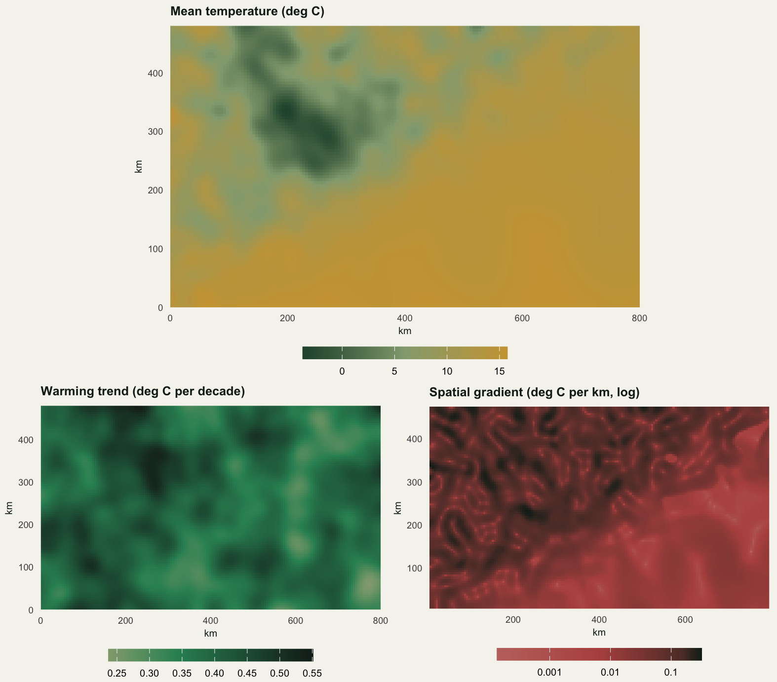
Almost all of the variation is in the denominator
The three panels above have the argument in them but not the number. The number is a coefficient of variation for each of the three quantities, and a decomposition of the variance of the log velocity, which is exact because the log of a ratio is a difference of logs:
\[\log V = \log b - \log G, \qquad \mathrm{var}(\log V) = \mathrm{var}(\log b) + \mathrm{var}(\log G) - 2\,\mathrm{cov}(\log b, \log G)\]
lv <- log(as.vector(V)); lb <- log(as.vector(B)); lg <- log(as.vector(G))

round(c(cv_of_the_trend = sd(B) / mean(B),
        cv_of_the_gradient = sd(G) / mean(G),
        cv_of_the_velocity = sd(V) / mean(V),
        var_log_velocity = var(lv),
        var_log_trend = var(lb),
        var_log_gradient = var(lg),
        minus_twice_covariance = -2 * cov(lb, lg),
        gradient_term_over_trend_term = var(lg) / var(lb),
        correlation_log_velocity_log_gradient = cor(lv, lg),
        correlation_log_velocity_trend = cor(lv, as.vector(B)),
        correlation_log_velocity_log_trend = cor(lv, lb)), 4)
cv_of_the_trend cv_of_the_gradient
0.1279 0.9521
cv_of_the_velocity var_log_velocity
2.2381 1.4575
var_log_trend var_log_gradient
0.0171 1.5397
minus_twice_covariance gradient_term_over_trend_term
-0.0993 90.0727
correlation_log_velocity_log_gradient correlation_log_velocity_trend
-0.9947 -0.2131
correlation_log_velocity_log_trend
-0.2061 The coefficient of variation of the trend is 0.1279, of the gradient 0.9521, of the velocity 2.2381. The velocity inherits the gradient’s spread and then some, because the gradient sits in the denominator: the cells where it nearly vanishes become the long upper tail of the velocity.
The variance decomposition is blunter. The log gradient contributes 1.5397 to the variance of the log velocity and the log trend 0.0171, with a covariance term of -0.0993 bringing the total to 1.4575: a ratio of 90 to one between the two contributions. Log velocity correlates with log gradient at -0.9947 and with the trend at -0.2131. A map of climate velocity is, to a very close approximation, a map of the reciprocal of the spatial temperature gradient, and the spatial temperature gradient is a map of the ground.
That is not a defect of the metric. It is what the metric says, and the dependence of exposure on the shape of the ground is the subject of Ackerly and colleagues in 2010 rather than a discovery of this post. But it changes what the map is evidence for. The plain in the south east is fast because it is flat: the nearest place that is a degree cooler than the middle of the plain is a long way off, so the isotherm has a long way to travel. The mountain is slow because a degree of cooling is 153.85 vertical metres up the slope. The difference between the two reserves is a difference in the shape of the ground, and the warming rate they experience is nearly the same.
# a ramp that never approaches the page colour: the lightest step is a gold
# darkened towards ink, and the colours are anchored on velocities rather than
# spread evenly, so the plain does not collapse into one flat tone
vel_cols <- c(te_pal$forest, te_pal$green, shade(te_pal$gold, 0.25),
              te_pal$clay)
lgV <- log10(as.vector(V))
vel_at <- (log10(c(min(V), 1, 12, max(V))) - min(lgV)) / diff(range(lgV))
vb <- c(0.03, 0.1, 0.3, 1, 3, 10, 30, 100)

ggplot(map_df(log10(V), 1), aes(x, y)) +
  geom_raster(aes(fill = z)) +
  geom_contour(data = map_df(elev), aes(x, y, z = z),
               breaks = 600, colour = te_pal$ink, linewidth = 0.3,
               linetype = 2) +
  geom_contour(data = map_df(elev), aes(x, y, z = z),
               breaks = 1400, colour = te_pal$ink, linewidth = 0.7) +
  coord_fixed(expand = FALSE) +
  scale_fill_gradientn(colours = vel_cols, values = vel_at,
                       name = "Climate velocity\n(km per year)",
                       breaks = log10(vb), labels = as.character(vb)) +
  labs(x = "Easting (km)", y = "Northing (km)",
       title = "The velocity map is a terrain map",
       subtitle = "Thin dashed contour 600 m, thick solid contour 1400 m") +
  theme_te() +
  theme(plot.subtitle = element_text(size = 9, colour = te_pal$ink),
        legend.position = "right",
        legend.title = element_text(size = 8.5),
        legend.key.width = grid::unit(0.45, "cm"),
        legend.key.height = grid::unit(1.5, "cm"))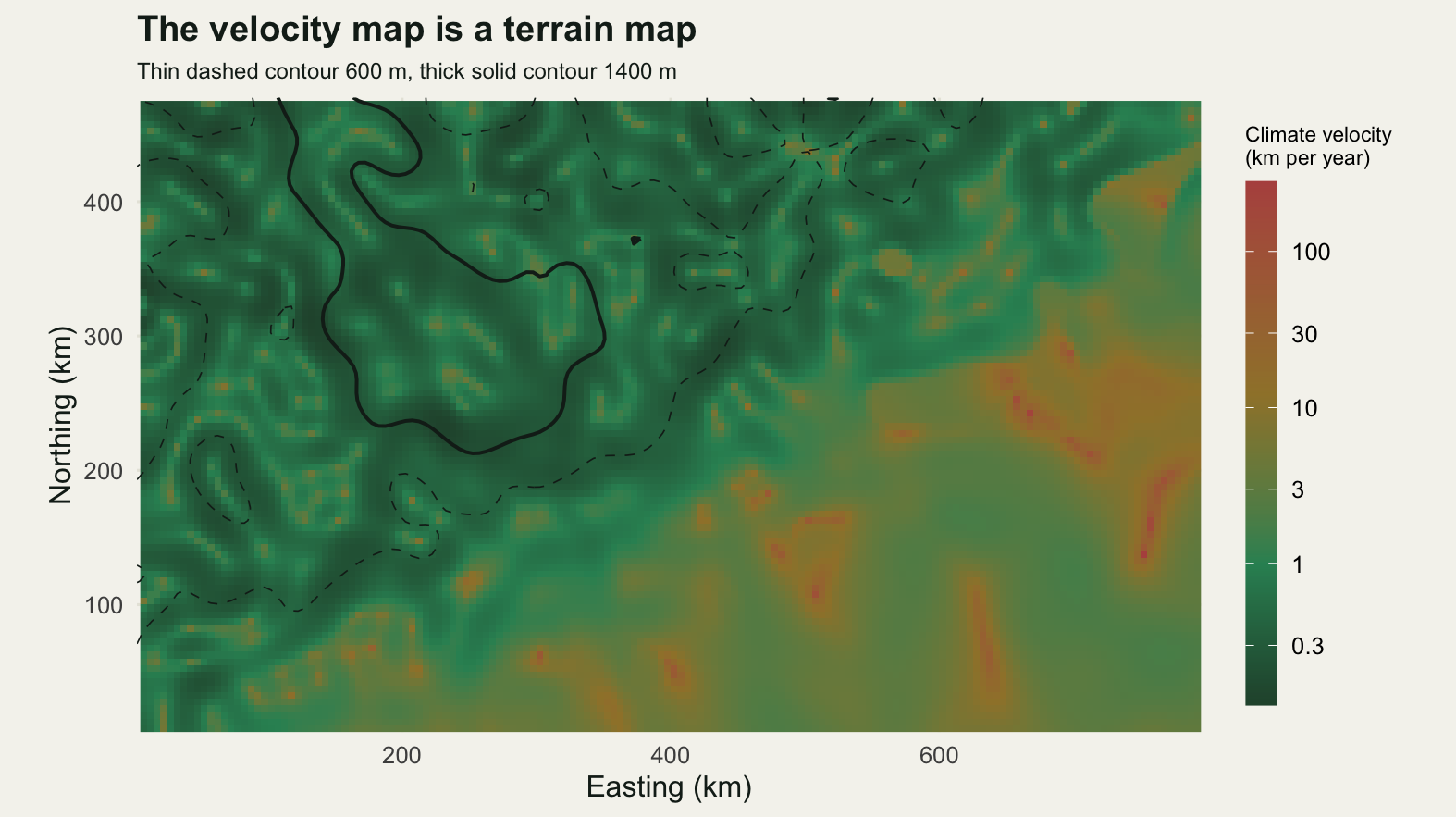
The mean is a statement about your flooring rule
Where the spatial gradient approaches zero the velocity diverges. This is not a numerical accident to be tidied away, it is the definition: if nowhere near by is any cooler, the distance an isotherm travels per year is unbounded. Every implementation therefore has to decide what to do about it, and the usual decision is a floor, a smallest gradient below which the gradient is replaced by the floor. The floor is rarely reported.
vs <- sort(as.vector(V), decreasing = TRUE)
top1 <- round(0.01 * length(vs))

round(c(velocity_median = median(V),
        velocity_mean = mean(V),
        mean_over_median = mean(V) / median(V),
        velocity_75th_percentile = quantile(V, 0.75),
        velocity_95th_percentile = quantile(V, 0.95),
        velocity_99th_percentile = quantile(V, 0.99),
        velocity_maximum = max(V),
        cells_in_the_top_one_percent = top1,
        share_of_the_total_held_by_them = sum(vs[1:top1]) / sum(vs),
        mean_after_dropping_the_single_fastest_cell = mean(vs[-1])), 4)
velocity_median
0.9042
velocity_mean
2.5235
mean_over_median
2.7909
velocity_75th_percentile.75%
2.8103
velocity_95th_percentile.95%
9.4990
velocity_99th_percentile.99%
19.8311
velocity_maximum
278.8241
cells_in_the_top_one_percent
149.0000
share_of_the_total_held_by_them
0.1530
mean_after_dropping_the_single_fastest_cell
2.5049 floors <- c(0, 0.001, 0.005, 0.02, 0.05)
sweep_mean <- sapply(floors, function(f)
mean(as.vector(B) / pmax(as.vector(G), f)))
sweep_med <- sapply(floors, function(f)
median(as.vector(B) / pmax(as.vector(G), f)))
sweep_hit <- sapply(floors, function(f) sum(as.vector(G) < f))
tab <- rbind(floor_C_per_km = floors, mean_velocity = sweep_mean,
median_velocity = sweep_med, cells_floored = sweep_hit,
percent_floored = 100 * sweep_hit / length(V))
colnames(tab) <- paste0("f", seq_along(floors))
print(round(tab, 4)) f1 f2 f3 f4 f5
floor_C_per_km 0.0000 0.0010 0.0050 0.0200 0.0500
mean_velocity 2.5235 2.4371 1.9879 1.0946 0.5981
median_velocity 0.9042 0.9042 0.9042 0.9042 0.6598
cells_floored 0.0000 38.0000 1071.0000 5502.0000 7997.0000
percent_floored 0.0000 0.2559 7.2112 37.0455 53.8446round(c(largest_mean_in_the_sweep = max(sweep_mean),
smallest_mean_in_the_sweep = min(sweep_mean),
ratio_of_the_two = max(sweep_mean) / min(sweep_mean),
largest_median_in_the_sweep = max(sweep_med),
smallest_median_in_the_sweep = min(sweep_med),
median_ratio = max(sweep_med) / min(sweep_med)), 4) largest_mean_in_the_sweep smallest_mean_in_the_sweep
2.5235 0.5981
ratio_of_the_two largest_median_in_the_sweep
4.2194 0.9042
smallest_median_in_the_sweep median_ratio
0.6598 1.3703 The median velocity is 0.9042 km per year and the mean is 2.5235, a ratio of 2.7909. The 95th percentile is 9.4990 and the 99th is 19.8311; the largest cell is 278.82 km per year, which is not a speed any organism or any isotherm meaningfully travels, it is one cell where the denominator nearly cancelled. The top one per cent of cells, 149 of them, hold 15.30 per cent of the summed velocity.
Now the sweep. With no floor at all the mean is 2.5235 km per year. At a floor of 0.02 degrees per km it is 1.0946, and at 0.05 it is 0.5981. Largest over smallest is 4.2194. The median does not move at all until the last step in the sweep, where a floor of 0.05 degrees per km is applied to 53.84 per cent of the map and starts reaching cells near the middle of the distribution; across the whole sweep the median changes by a factor of 1.3703 against 4.2194 for the mean.
So a mean climate velocity, quoted for a region, is partly a statement about the author’s flooring rule, and a comparison of mean velocities between two studies that floored differently is not a comparison of anything. Report the median, or a quantile, and say what you did about the pole. This is the same reasoning that makes a median a better summary of any positive skewed quantity, and it bites harder here because the skew is not a property of the data, it is a property of division.
fl <- c(0.0002, 0.0005, 0.001, 0.002, 0.005, 0.01, 0.02, 0.05)
fl_mean <- sapply(fl, function(f) mean(as.vector(B) / pmax(as.vector(G), f)))
fl_med <- sapply(fl, function(f) median(as.vector(B) / pmax(as.vector(G), f)))
sw <- data.frame(floor = rep(fl, 2), value = c(fl_mean, fl_med),
                 stat = rep(c("Mean", "Median"), each = length(fl)))

p_hist <- ggplot(data.frame(v = log10(as.vector(V))), aes(v)) +
  geom_histogram(bins = 46, fill = te_pal$sage, colour = te_pal$forest,
                 linewidth = 0.2) +
  geom_vline(xintercept = log10(median(V)), colour = te_pal$forest,
             linewidth = 0.9) +
  geom_vline(xintercept = log10(mean(V)), colour = te_pal$clay,
             linewidth = 0.9, linetype = 2) +
  # centring a label on its own vertical line puts the line through the middle
  # of the word: each label sits beside its line instead, on the side that
  # keeps the two of them apart, and both sit at the same height
  annotate("text", x = log10(median(V)), y = Inf, label = "median",
           hjust = 1.1, vjust = 1.7, size = 3.1, colour = te_pal$forest) +
  annotate("text", x = log10(mean(V)), y = Inf, label = "mean",
           hjust = -0.1, vjust = 1.7, size = 3.1, colour = te_pal$clay) +
  scale_x_continuous(breaks = log10(c(0.3, 3, 30)),
                     labels = c("0.3", "3", "30")) +
  labs(x = "Climate velocity (km per year)", y = "Cells",
       title = "Velocity across the map") +
  theme_te() +
  theme(plot.title = element_text(size = 10))

p_sweep <- ggplot(sw, aes(floor, value, colour = stat, shape = stat)) +
  geom_line(linewidth = 0.9) +
  geom_point(size = 2.4) +
  annotate("text", x = fl[3], y = fl_mean[3], label = "Mean", vjust = -1.3,
           size = 3.3, colour = te_pal$clay) +
  annotate("text", x = fl[3], y = fl_med[3], label = "Median", vjust = 2.0,
           size = 3.3, colour = te_pal$forest) +
  scale_x_log10(breaks = c(0.0002, 0.001, 0.005, 0.02, 0.05),
                labels = c("0.0002", "0.001", "0.005", "0.02", "0.05")) +
  scale_colour_manual(values = c(te_pal$clay, te_pal$forest), guide = "none") +
  scale_shape_manual(values = c(17, 16), guide = "none") +
  labs(x = "Gradient floor (deg C per km)", y = "Velocity (km per year)",
       title = "The mean moves, the median does not") +
  theme_te() +
  theme(plot.title = element_text(size = 10))

lay_row(list(p_hist, p_sweep))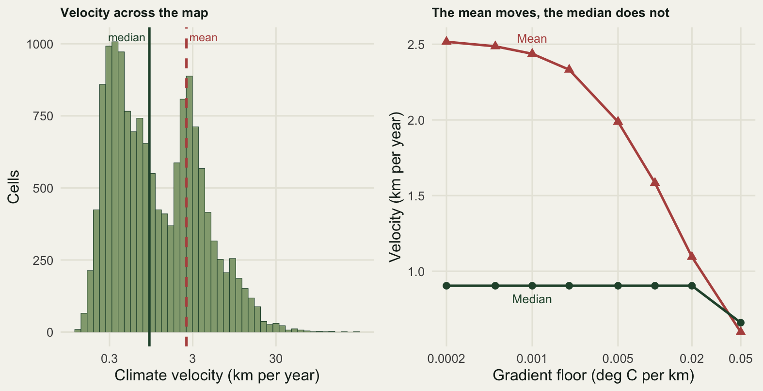
Velocity is not scale free
The gradient is a finite difference over one cell width, so it is a property of the grid as much as of the climate. Coarsen the grid and the same landscape has smaller gradients, because averaging over a larger block flattens the surface before the difference is taken. Whether that raises or lowers the velocity, and by how much in which sort of terrain, is a measurement rather than an argument.
Aggregating the trend map is legitimate here without recomputing anything, because the slope operator is linear: the trend of a block mean series is the block mean of the trends. The chunk checks that rather than asserting it.
agg <- function(M, f) {
  if (f == 1) return(M)
  apply(array(M, c(f, nrow(M) %/% f, f, ncol(M) %/% f)), c(2, 4), mean)
}
grad_full <- function(M, d) {
  Mp <- rbind(M[1, ], M, M[nrow(M), ])
  grad_mag(cbind(Mp[, 1], Mp, Mp[, ncol(Mp)]), d)
}

Bfull <- matrix(trend, nx, ny)
agg_then_trend <- as.vector(sapply(seq_len(n_year), function(k)
  as.vector(agg(matrix(Y[, k], nx, ny), 2))) %*% w)
round(c(aggregate_then_fit_minus_fit_then_aggregate =
          max(abs(agg_then_trend - as.vector(agg(Bfull, 2))))), 10)
aggregate_then_fit_minus_fit_then_aggregate
0 roughness <- grad_full(elev, cell_km) # metres of elevation per km
grain <- c(1, 2, 4, 8)
gr <- t(sapply(grain, function(f) {
Tc <- agg(Tm, f)
Vc <- as.vector(inner(agg(Bfull, f)) / grad_mag(Tc, cell_km * f))
rc <- as.vector(inner(agg(roughness, f)))
q <- quantile(rc, c(0.25, 0.75))
flat <- median(Vc[rc <= q[1]]); rough <- median(Vc[rc >= q[2]])
c(cell_km = cell_km * f, cells = length(Vc),
median_gradient = median(grad_mag(Tc, cell_km * f)),
median_velocity = median(Vc), mean_velocity = mean(Vc),
flattest_quartile = flat, roughest_quartile = rough,
flat_over_rough = flat / rough)
}))
rownames(gr) <- paste0("grain_", grain)
print(round(gr, 4)) cell_km cells median_gradient median_velocity mean_velocity
grain_1 5 14852 0.0425 0.9042 2.5235
grain_2 10 3588 0.0395 0.9569 2.5417
grain_4 20 836 0.0345 1.1127 2.7515
grain_8 40 180 0.0306 1.3336 2.8030
flattest_quartile roughest_quartile flat_over_rough
grain_1 3.8364 0.2848 13.4722
grain_2 3.8027 0.3065 12.4085
grain_4 3.7303 0.3922 9.5116
grain_8 4.2154 0.6553 6.4329round(c(median_velocity_at_40_km_over_5_km =
gr[4, "median_velocity"] / gr[1, "median_velocity"],
percent_rise_in_median_velocity =
100 * (gr[4, "median_velocity"] / gr[1, "median_velocity"] - 1),
median_gradient_at_5_km_over_40_km =
gr[1, "median_gradient"] / gr[4, "median_gradient"],
terrain_contrast_at_5_km = gr[1, "flat_over_rough"],
terrain_contrast_at_40_km = gr[4, "flat_over_rough"],
roughest_quartile_at_40_km_over_5_km =
gr[4, "roughest_quartile"] / gr[1, "roughest_quartile"],
flattest_quartile_at_40_km_over_5_km =
gr[4, "flattest_quartile"] / gr[1, "flattest_quartile"]), 4) median_velocity_at_40_km_over_5_km percent_rise_in_median_velocity
1.4749 47.4875
median_gradient_at_5_km_over_40_km terrain_contrast_at_5_km
1.3904 13.4722
terrain_contrast_at_40_km roughest_quartile_at_40_km_over_5_km
6.4329 2.3012
flattest_quartile_at_40_km_over_5_km
1.0988 Aggregating first and fitting second gives the same trends as fitting first and aggregating second, to ten decimal places, so the shortcut is exact and not an approximation.
The median gradient falls from 0.0425 degrees per km at 5 km cells to 0.0306 at 40 km cells, a factor of 1.3904, and the median velocity rises from 0.9042 to 1.3336 km per year. Coarsening the grid makes the climate appear to move faster, by 47.49 per cent over this range of grains. A velocity computed on a 5 km grid and a velocity computed on a 40 km grid are two different quantities with the same name, and comparing them across studies is not a comparison of climates.
The terrain contrast goes the same way and it is the more useful number. Splitting the map by the roughness of the underlying ground, the flattest quartile has a median velocity 13.4722 times the roughest quartile at 5 km cells and 6.4329 times at 40 km cells. Coarsening compresses the contrast, because it takes more gradient away from rough ground than from flat ground: the roughest quartile’s median velocity rises steadily from 0.2848 to 0.6553, a factor of 2.3012, while the flattest quartile’s goes 3.8364, 3.8027, 3.7303, 4.2154: down slightly, then up, with no clear direction over a factor of 1.0988 in total.
I had expected the flat quartile to move the more of the two, on the reasoning that smoothing should cancel the small-scale wiggles that give the plain its extreme cells. It does not, and the reason is in the way the plain’s gradient is built. On the plain the gradient is mostly the latitudinal term, which is a constant and survives any amount of averaging; in the mountains it is relief, which does not. That generalises past this simulation. Coarsening erodes whatever part of the gradient has short spatial scale and leaves whatever part is regional, so mountain refugia get less mountainous with every step of aggregation and a latitudinal gradient does not care.
The analogue velocity, and the climates with no analogue
The gradient method is local. It differentiates the surface at a cell and asks how fast the isotherm through that cell is sliding, and it has no idea what is over the next ridge. The distance-based alternative, the climate analogue velocity, is not local: for each cell it searches the whole domain for a place whose climate matches, and reports the distance divided by the time step. Hamann and colleagues set the two side by side in 2015 and the difference is not cosmetic.
There are two directions and they answer different questions. Forward velocity starts from a cell’s present climate and asks how far you must travel to reach a place that will have that climate in the future: it is the distance a resident species would have to cover. Backward velocity starts from a cell’s future climate and asks where, at present, that climate exists: it is the distance the future occupants have to come. This post uses forward velocity as the comparison, because it is the one that matches what a velocity is usually read as, and reports the backward count as well because it is the one that finds the climates with no present analogue.
The search is a nearest-neighbour distance under a constraint, done in blocks so that no full distance matrix between all pairs of cells has to be held at once. Building distances across a surface in base R also comes up in least-cost paths and resistance, where the distance is a cost rather than a straight line; here it is a straight line, which is the generous assumption.
horizon <- 50
tol <- 0.25

present <- as.vector(Tm)
future <- present + as.vector(Bfull) * horizon
xx <- as.vector(gx); yy <- as.vector(gy)
idx <- as.vector(inner(matrix(seq_len(nx * ny), nx, ny)))

fwd <- rep(NA_real_, length(idx))
bwd <- rep(NA_real_, length(idx))
for (ch in split(seq_along(idx), ceiling(seq_along(idx) / 250))) {
  ii <- idx[ch]
  D <- sqrt(outer(xx[ii], xx, "-")^2 + outer(yy[ii], yy, "-")^2)
  Df <- D; Df[abs(outer(present[ii], future, "-")) > tol] <- Inf
  Db <- D; Db[abs(outer(future[ii], present, "-")) > tol] <- Inf
  fwd[ch] <- apply(Df, 1, min)
  bwd[ch] <- apply(Db, 1, min)
}

v_ana <- fwd / horizon
has <- is.finite(v_ana)
v_grad <- as.vector(V)
rgh <- as.vector(inner(roughness)); elv <- as.vector(inner(elev))
qr <- quantile(rgh, c(0.25, 0.75))

round(c(horizon_years = horizon, tolerance_C = tol,
        smallest_analogue_step_km_per_year = cell_km / horizon,
        cells_with_no_forward_analogue = sum(!has),
        percent_with_no_forward_analogue = 100 * mean(!has),
        cells_with_no_backward_analogue = sum(!is.finite(bwd)),
        percent_with_no_backward_analogue = 100 * mean(!is.finite(bwd)),
        lowest_elevation_with_no_forward_analogue_m = min(elv[!has]),
        mean_elevation_of_those_cells_m = mean(elv[!has]),
        mean_elevation_of_the_map_m = mean(elv)), 4)
horizon_years
50.0000
tolerance_C
0.2500
smallest_analogue_step_km_per_year
0.1000
cells_with_no_forward_analogue
80.0000
percent_with_no_forward_analogue
0.5386
cells_with_no_backward_analogue
4207.0000
percent_with_no_backward_analogue
28.3262
lowest_elevation_with_no_forward_analogue_m
2329.9042
mean_elevation_of_those_cells_m
2435.9695
mean_elevation_of_the_map_m
471.6200 round(c(spearman_correlation_of_the_two_maps =
cor(v_grad[has], v_ana[has], method = "spearman"),
gradient_median = median(v_grad[has]),
analogue_median = median(v_ana[has]),
gradient_99th = quantile(v_grad[has], 0.99),
analogue_99th = quantile(v_ana[has], 0.99),
gradient_max = max(v_grad[has]), analogue_max = max(v_ana[has]),
flattest_quartile_gradient = median(v_grad[rgh <= qr[1]]),
flattest_quartile_analogue = median(v_ana[rgh <= qr[1] & has]),
roughest_quartile_gradient = median(v_grad[rgh >= qr[2]]),
roughest_quartile_analogue = median(v_ana[rgh >= qr[2] & has]),
terrain_contrast_gradient_method =
median(v_grad[rgh <= qr[1]]) / median(v_grad[rgh >= qr[2]]),
terrain_contrast_analogue_method =
median(v_ana[rgh <= qr[1] & has]) / median(v_ana[rgh >= qr[2] & has]),
contrast_gradient_over_analogue =
(median(v_grad[rgh <= qr[1]]) / median(v_grad[rgh >= qr[2]])) /
(median(v_ana[rgh <= qr[1] & has]) /
median(v_ana[rgh >= qr[2] & has])),
median_gradient_velocity_of_the_no_analogue_cells =
median(v_grad[!has]),
percent_of_analogue_cells_within_two_grid_steps =
100 * mean(v_ana[has] <= 2 * cell_km / horizon)), 4) spearman_correlation_of_the_two_maps
0.7629
gradient_median
0.9104
analogue_median
0.8544
gradient_99th.99%
19.9050
analogue_99th.99%
5.5946
gradient_max
278.8241
analogue_max
6.4885
flattest_quartile_gradient
3.8364
flattest_quartile_analogue
2.6571
roughest_quartile_gradient
0.2848
roughest_quartile_analogue
0.3000
terrain_contrast_gradient_method
13.4722
terrain_contrast_analogue_method
8.8569
contrast_gradient_over_analogue
1.5211
median_gradient_velocity_of_the_no_analogue_cells
0.4836
percent_of_analogue_cells_within_two_grid_steps
2.1933 The two maps agree in rank at a Spearman correlation of 0.7629, which is high enough that a reader glancing at both would call them the same map and low enough that the disagreement is worth locating. It is in the tails and in the terrain. Over the cells that have an analogue, so that the two are computed on the same set, the gradient method’s 99th percentile is 19.9050 km per year and its maximum 278.82; the analogue method’s 99th percentile is 5.5946 and its maximum 6.4885. The pole is gone, because the analogue method only ever divides by the fixed horizon: the furthest a cell can have to look is the size of the domain.
By terrain, the flattest quartile of the map has a median gradient velocity of 3.8364 km per year and a median analogue velocity of 2.6571, so the local derivative overstates the plain. The roughest quartile has 0.2848 against 0.3000, so the local derivative understates the mountain. The contrast between flat and rough is 13.4722 by the gradient method and 8.8569 by the analogue method. Both say the plain moves faster. The gradient method says it 1.5211 times as strongly, and the difference is a real disagreement about the mountain: a local derivative knows how steep the slope is at the cell and does not know that the slope ends.
Then the part the gradient method cannot say at all. 80 cells, or 0.5386 per cent of the map, have no forward analogue anywhere in the domain: no place, at the end of the horizon, will be as cool as they are now. Every one of them is above 2329.90 m, and their mean elevation is 2435.97 m against 471.62 m for the map. Their median gradient velocity is 0.4836 km per year, which is slow, which on a gradient velocity map reads as safe. That is the mountaintop failure in one number: a summit has a steep local gradient, so the isotherm through it moves slowly across the ground, and the gradient method scores it as a refuge right up to the point where the isotherm leaves the top of the mountain and there is nowhere left for it to be.
The other direction is larger. 4207 cells, 28.3262 per cent of the map, have no backward analogue: their future climate does not exist anywhere in the domain today. Those are the novel climates, and they are in the warm lowlands rather than on the summits. Neither number is visible anywhere in a gradient velocity map.
ana_m <- matrix(v_ana, nrow(V), ncol(V))
ana_m[!is.finite(ana_m)] <- NA

d4 <- rbind(cbind(map_df(log10(V), 1), method = "Gradient method"),
            cbind(map_df(log10(ana_m), 1),
                  method = "Forward analogue method"))
d4$method <- factor(d4$method, levels = c("Gradient method",
                                          "Forward analogue method"))

# the no-analogue cells are a class, not a value, so they get a neutral grey
# that is nowhere on the velocity ramp and a legend key of their own
no_ana <- d4[is.na(d4$z), ]
no_ana$key <- "No analogue in the domain"
grey_off <- "#8c8c8c"

ggplot(d4, aes(x, y)) +
  geom_raster(aes(fill = z)) +
  geom_tile(data = no_ana, aes(colour = key), fill = grey_off,
            linewidth = 0) +
  facet_wrap(~method) +
  coord_fixed(expand = FALSE) +
  scale_fill_gradientn(colours = vel_cols, values = vel_at,
                       name = "Climate velocity (km per year)",
                       breaks = log10(vb), labels = as.character(vb),
                       na.value = grey_off,
                       guide = guide_colourbar(title.position = "top",
                                               title.hjust = 0.5, order = 1)) +
  scale_colour_manual(name = NULL,
                      values = c("No analogue in the domain" = grey_off),
                      guide = guide_legend(
                        order = 2,
                        override.aes = list(fill = grey_off,
                                            colour = te_pal$ink,
                                            linewidth = 0.3))) +
  labs(x = "Easting (km)", y = "Northing (km)",
       title = "The analogue method compresses the terrain contrast") +
  theme_te() +
  theme(strip.text = element_text(colour = te_pal$ink, face = "bold",
                                  size = 9),
        legend.key.width = grid::unit(1.5, "cm"),
        legend.key.height = grid::unit(0.3, "cm"))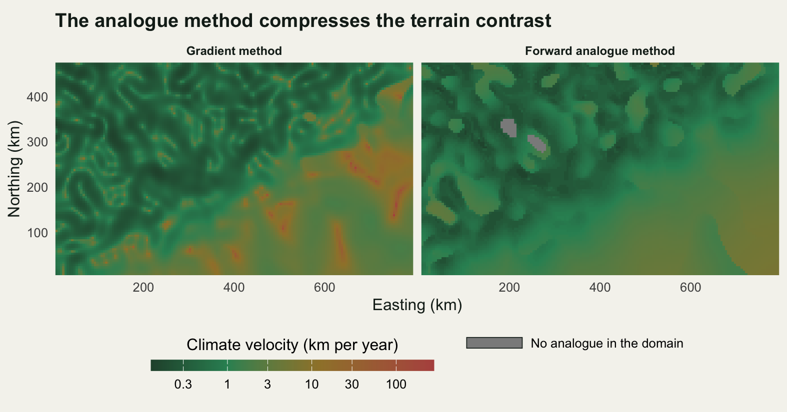
The honest limit
Climate velocity is a property of the climate surface and of nothing else. There is no dispersal ability in it, no habitat, no soil, no barrier, no competitor, no biology of any kind. Two species sharing a cell get the same velocity and have entirely different problems: a wind-dispersed annual with a seed shadow of a hundred metres per generation and a bird that moves a hundred kilometres in a week are told the same number. The velocity is the speed of the target, not the speed of the thing chasing it, and a comparison between the two is the analysis, not this.
The second limit is the tolerance in the analogue calculation. The 0.25 degree window and the 50 year horizon are choices, and a wide enough window would give every cell counted here as having no analogue an analogue. The analogue velocity is also quantised by the grid: the smallest non-zero value it can return is one cell width over the horizon, 0.10 km per year. On this grid that bites on only 2.1933 per cent of the cells with an analogue, the ones sitting within two cells of the floor, but the floor scales with the cell width, so on a 50 km grid the same calculation would be reporting the grid over much of the map.
The third is that everything here uses one climate variable. Real climates are at least two dimensional, temperature and water, and a cell can have a close temperature analogue and no precipitation analogue in the same place, a point made carefully by Garcia and colleagues in 2014. The direction of that error is not in doubt, because adding a second variable to the search can only remove candidate cells and never add them: the no-analogue count computed here is a lower bound on what a two-variable search would give on the same surface.
And a fourth, about the map rather than the metric. The velocity map here is computed on a simulated surface with no measurement error in the temperature field. A real gridded climatology is interpolated, its interpolation is smoother than the ground in exactly the places where the gradient matters most, and the smoothing raises velocity in mountains by flattening them. Interpolating carefully is a separate job, and kriging and spatial interpolation covers what the smoothing does to the surface before any of this arithmetic starts.
Where to go next
The measurement this post does not do is the biological one. Velocity is a prediction about the speed a species would need; the observed shift is what happened. Putting the two together, and the lag between them, is range shifts and the climate lag, and the failure modes of that comparison, which are mostly about detection and about the elevation an observer walks to, are in checking a range shift analysis. Read that pair before quoting a velocity as an exposure metric for a species.
For the physiological side of exposure, which is a different quantity computed from the same climate data, thermal safety margins and warming measures how much headroom an organism has above its current temperature, and degree days and thermal time measures the accumulated warmth that actually drives development. A velocity is a property of the target; those two are properties of the organism standing in front of it, and a reserve is not ranked by any one of the three.
Two spatial neighbours are worth reading for the machinery rather than the ecology. Raster basics with terra is where the file handling and the projections live once the arithmetic is understood, and it matters here because a velocity computed on cells that are not equal-area is wrong by the ratio of the cell dimensions. Spatial autocorrelation and Moran’s I is the tool for the obvious next question about any of these maps, which is how many independent cells there really are in it, and the answer for a velocity map is a great deal fewer than the cell count.
References
Loarie SR, Duffy PB, Hamilton H, Asner GP, Field CB, Ackerly DD 2009 Nature 462(7276):1052-1055 (10.1038/nature08649)
Ackerly DD, Loarie SR, Cornwell WK, Weiss SB, Hamilton H, Branciforte R, Kraft NJB 2010 Diversity and Distributions 16(3):476-487 (10.1111/j.1472-4642.2010.00654.x)
Burrows MT, Schoeman DS, Buckley LB, Moore P, Poloczanska ES, Brander KM, Brown C, Bruno JF, Duarte CM, Halpern BS, Holding J, Kappel CV, Kiessling W, O’Connor MI, Pandolfi JM, Parmesan C, Schwing FB, Sydeman WJ, Richardson AJ 2011 Science 334(6056):652-655 (10.1126/science.1210288)
Dobrowski SZ, Abatzoglou JT, Swanson AK, Greenberg JA, Mynsberge AR, Holden ZA, Schwartz MK 2013 Global Change Biology 19(1):241-251 (10.1111/gcb.12026)
Garcia RA, Cabeza M, Rahbek C, Araujo MB 2014 Science 344(6183):1247579 (10.1126/science.1247579)
Hamann A, Roberts DR, Barber QE, Carroll C, Nielsen SE 2015 Global Change Biology 21(2):997-1004 (10.1111/gcb.12736)