library(ggplot2)

te_paper  <- "#f5f4ee"
te_ink    <- "#16241d"
te_body   <- "#2c3a31"
te_forest <- "#275139"
te_rust   <- "#b5534e"
te_gold   <- "#c9b458"
te_line   <- "#dad9ca"

theme_datasheet <- function() {
  theme_minimal(base_size = 12) +
    theme(plot.background  = element_rect(fill = te_paper, colour = NA),
          panel.background = element_rect(fill = te_paper, colour = NA),
          panel.grid.major = element_line(colour = te_line, linewidth = 0.3),
          panel.grid.minor = element_blank(),
          text             = element_text(colour = te_body),
          plot.title       = element_text(colour = te_ink, face = "bold"),
          plot.subtitle    = element_text(colour = te_body),
          axis.text        = element_text(colour = te_body),
          strip.text       = element_text(colour = te_ink))
}Additive or compensatory harvest mortality
R
survival analysis
harvest
measurement error
simulation
ecology tutorial
Regressing annual survival on the kill rate of the same collared animals manufactures additive harvest mortality. Closed form, false rate and a noisy fix in R.
A game agency has put radio collars on thirty adult birds of a hunted species every spring for fifteen years. Each winter it counts how many of the thirty were still alive a year later, how many were shot, and how many died of something else. The season length has varied from year to year, so the share shot has varied too, and the obvious analysis is to put the fifteen annual survival rates on the vertical axis and the fifteen kill rates on the horizontal one and fit a line. A clearly negative slope reads as additive harvest mortality: every bird shot is a bird that would otherwise have lived. A flat line reads as compensation: the shot birds would have died anyway.
That test has a known flaw, and this post measures it rather than discovering it. The survival rate and the kill rate of a year are estimated from the same thirty animals, so they are two cells of one multinomial count and their sampling errors are negatively correlated: a year in which chance put a few more birds in front of hunters is, by the same draw, a year in which fewer were left to survive. That covariance tilts the fitted line downwards even when harvest has no effect on survival at all. Servanty and colleagues (2010) name two difficulties with estimating the relationship between cause-specific mortalities from marked animals: an intrinsic bias that depends on natural survival in the absence of the competing cause, and sampling variation that has to be separated from the process correlation. Both show up below, the first as a closed form with no noise in it and the second as a covariance that can be written down exactly. What the post adds is the size of each in a known-fate telemetry design, the rate at which the naive test declares additivity when compensation is complete, and what the textbook moment correction costs.
The two hypotheses are already on this site as competing models. Adaptive management and learning keeps an additive and a threshold compensatory survival multiplier side by side and learns their relative weight from spring counts; it never estimates the strength of the relationship from marked animals. Stochastic dynamic programming for harvest has no survival hypotheses at all: it sets the growth parameters of a fished stock rather than fitting them and derives the harvest rule that follows. Both treat the response to harvest as something to act on. This post is about how it gets measured.
The statistical ingredients are also on the site, each in a different setting. Competing risks and cumulative incidence shows that the share of animals dying of one cause depends on the other causes competing with it; that is where the intrinsic bias comes from. Measurement error and regression dilution treats independent error in a predictor and ends on the observation that attenuation cannot manufacture an effect, only weaken a real one. That is true of independent error and false here, because the error in the kill rate is correlated with the error in the response. The Gompertz state-space model meets sampling error in a population time series: noisy counts used as the predictor of next year’s count pull the density-dependence slope towards zero and make a population look more tightly regulated than it is. That is dilution of a real slope by independent error; here the error is shared between the two axes of the same year. Errors-in-variables and Deming regression handles error on both axes but draws the two errors independently, and its variance ratio has no place for a covariance.
Two hypotheses written as hazards
Each year has a natural mortality hazard and a harvest hazard acting at the same time, the continuous-time competing-risks formulation that Lebreton (2005) uses for exploited populations. The harvest hazard of a year is drawn uniformly between 0.02 and 0.20, standing in for regulations that change from year to year. Under the additive hypothesis the natural hazard is 0.25 every year, so the total hazard is 0.25 plus the harvest hazard. Under full compensation the natural hazard is 0.25 minus the harvest hazard, so the total hazard is 0.25 in every year and harvest only changes which cause an animal dies of. Every one of these values was fixed before anything was run.
Survival over the year is the exponential of minus the total hazard. The probability of being shot is the harvest share of the total hazard times the probability of dying at all, which is the cumulative incidence of the harvest cause. Burnham and Anderson (1984) wrote a completely additive and a completely compensatory survival model for band-recovery data and told them apart by comparing their maximised log-likelihoods. The continuum between the two is written here as S = S0 (1 - b K), with K the kill rate: b = 1 is additivity and b = 0 is full compensation. The shortcut examined in this post fits that form by least squares to the estimated annual rates: with a fitted line S = a + slope K, the estimate is b = -slope / a.
h_nat <- 0.25
h_lo  <- 0.02
h_hi  <- 0.20

fate_probs <- function(h_harv, truth, h_extra = 0) {
  h_natural <- if (truth == "additive") h_nat + 0 * h_harv else h_nat - h_harv
  h_tot  <- pmax(h_natural + h_extra, 0) + h_harv
  p_surv <- exp(-h_tot)
  list(s = p_surv, k = h_harv / h_tot * (1 - p_surv))
}

pop_moments <- function(truth, lo = h_lo, hi = h_hi) {
  e_of <- function(g) integrate(function(x) g(fate_probs(x, truth)) / (hi - lo),
                                lo, hi, rel.tol = 1e-11)$value
  list(es = e_of(function(p) p$s), ek = e_of(function(p) p$k),
       ekk = e_of(function(p) p$k^2), esk = e_of(function(p) p$s * p$k))
}

mom_add  <- pop_moments("additive")
var_k_add <- mom_add$ekk - mom_add$ek^2
slope_pop <- (mom_add$esk - mom_add$es * mom_add$ek) / var_k_add
b_pop     <- -slope_pop / (mom_add$es - slope_pop * mom_add$ek)
b_local   <- h_nat / (1 - exp(-h_nat))

h_fine    <- seq(h_lo, h_hi, length.out = 1e5)
p_fine    <- fate_probs(h_fine, "additive")
fit_fine  <- coef(lm(p_fine$s ~ p_fine$k))
b_grid    <- unname(-fit_fine[2] / fit_fine[1])

net_harv  <- 1 - exp(-h_fine)
stopifnot(all(p_fine$k < net_harv))
k_share   <- p_fine$k[5e4] / net_harv[5e4]
h_mid     <- h_fine[5e4]
s_comp    <- exp(-h_nat)

b_ls      <- function(k, s) { cf <- coef(lm(s ~ k)); unname(-cf[2] / cf[1]) }
b_before  <- b_ls(net_harv, s_comp * (1 - net_harv))
b_after   <- b_ls(s_comp * net_harv, s_comp - s_comp * net_harv)
stopifnot(abs(b_before - 1) < 1e-9, abs(b_after - 1 / s_comp) < 1e-9,
          b_before < b_pop, b_pop < b_after)
Under additivity with no sampling error at all, the least-squares regression of survival on kill rate across the design range gives b = 1.1252, computed by numerical integration over the uniform harvest hazard; a least-squares fit to 100000 equally spaced harvest hazards gives 1.1252. Neither is a simulation result. Under compensation survival is 0.7788 in every year, the slope is zero and b is zero.
The additive value is not one, and the reason is the competing risk. If harvest acted alone, a harvest hazard h would kill a share 1 - exp(-h), and survival would be S0 times one minus that share exactly, a straight line with b = 1. The observed kill rate is smaller, because some animals that would have been shot die of natural causes first: at a harvest hazard of 0.11 the kill rate is 0.887 times the net harvest share. Survival therefore falls by more per unit of observed kill than b = 1 allows. For a small harvest hazard the local value is h_nat / (1 - exp(-h_nat)) = 1.1302, and the curvature across the design range brings the regression value down slightly to 1.1252. This is the S-on-K counterpart of what Servanty and colleagues (2010) call an intrinsic bias: like theirs, it comes from the competing risk and depends on natural mortality in the absence of harvest, which a real study does not know, and it has nothing to do with sample size. That value belongs to hazards that act together all through the year, and the timing of the season moves it. If the whole harvest came before any natural mortality, the kill rate would be the net harvest share 1 - exp(-h) itself, survival would be S0 (1 - K), and the regression over the same design range gives b = 1.000. If it came after all natural mortality, only the S0 survivors could be shot, survival would be S0 - K, and b is 1 / S0 = 1.284. Concurrent hazards sit between these two extremes, and every simulation below uses them.
sim_studies <- function(n_anim, n_year, n_rep, truth, split = FALSE, sd_nat = 0) {
  h_harv <- matrix(runif(n_rep * n_year, h_lo, h_hi), n_rep, n_year)
  h_ext  <- if (sd_nat > 0) rnorm(n_rep * n_year, 0, sd_nat) else 0
  p_yr   <- fate_probs(h_harv, truth, h_ext)
  p_s    <- matrix(p_yr$s, n_rep, n_year)
  p_k    <- matrix(p_yr$k, n_rep, n_year)
  n_surv <- matrix(rbinom(n_rep * n_year, n_anim, p_s), n_rep, n_year)
  n_kill <- if (split) {
    matrix(rbinom(n_rep * n_year, n_anim, p_k), n_rep, n_year)
  } else {
    matrix(rbinom(n_rep * n_year, n_anim - n_surv, p_k / (1 - p_s)), n_rep, n_year)
  }
  s_hat <- n_surv / n_anim
  k_hat <- n_kill / n_anim
  s_bar <- rowMeans(s_hat)
  k_bar <- rowMeans(k_hat)
  s_cen <- s_hat - s_bar
  k_cen <- k_hat - k_bar
  sxx   <- rowSums(k_cen^2)
  sxy   <- rowSums(s_cen * k_cen)
  slope <- sxy / sxx
  icpt  <- s_bar - slope * k_bar
  se_sl <- sqrt(rowSums((s_cen - slope * k_cen)^2) / (n_year - 2) / sxx)
  v_k   <- rowMeans(k_hat * (1 - k_hat)) / (n_anim - 1)
  c_sk  <- -rowMeans(s_hat * k_hat) / (n_anim - 1)
  den   <- sxx / (n_year - 1) - v_k
  sl_c  <- (sxy / (n_year - 1) - c_sk) / den
  data.frame(b = -slope / icpt,
             t_val = slope / se_sl,
             b_bench = k_bar / (n_anim * sxx / (n_year - 1) + k_bar^2),
             b_c = ifelse(den > 0, -sl_c / (s_bar - sl_c * k_bar), NA))
}
The function simulates many studies at once. In each year the fates of the collared animals are one multinomial draw, generated as a binomial number of survivors followed by a binomial number shot among the animals that died. The naive slope, its standard error and b come from the least-squares formulas written out in matrix form, which gives the same numbers as lm() and is much faster. The lines from v_k to sl_c are the moment correction used later in the post, and b_bench is a benchmark that the reporting section uses. With split = TRUE the kill count comes from a second, independent group of the same size, a construction used as a control below.
n_small <- 30
t_small <- 15
set.seed(2210)
one_df <- do.call(rbind, lapply(c("additive", "compensatory"), function(tr) {
  h_harv <- runif(t_small, h_lo, h_hi)
  p_yr   <- fate_probs(h_harv, tr)
  n_surv <- rbinom(t_small, n_small, p_yr$s)
  n_kill <- rbinom(t_small, n_small - n_surv, p_yr$k / (1 - p_yr$s))
  data.frame(truth = tr, k_true = p_yr$k, s_true = p_yr$s,
             s_hat = n_surv / n_small, k_hat = n_kill / n_small)
}))
one_fit <- sapply(split(one_df, one_df$truth), function(d) {
  cf <- coef(summary(lm(s_hat ~ k_hat, data = d)))
  k_c <- d$k_hat - mean(d$k_hat)
  s_c <- d$s_hat - mean(d$s_hat)
  sl  <- sum(s_c * k_c) / sum(k_c^2)
  se  <- sqrt(sum((s_c - sl * k_c)^2) / (t_small - 2) / sum(k_c^2))
  stopifnot(abs(sl - cf[2, 1]) < 1e-12, abs(sl / se - cf[2, 3]) < 1e-9,
            abs(cf[2, 4] - 2 * pt(-abs(cf[2, 3]), t_small - 2)) < 1e-12)
  c(b = -cf[2, 1] / cf[1, 1], p_one = pt(cf[2, 3], t_small - 2))
})
The stopifnot() line checks that the matrix-form slope and t value match lm() on these two studies, and that the p value summary(lm()) prints is the two-sided one. One simulated study of each kind, drawn with 30 animals a year for 15 years, shows what the analyst sees. The additive study returns b = 1.08, and the compensatory study returns b = 0.53 with a one-sided p value for a negative slope of 0.018.
one_df$panel <- factor(one_df$truth, c("additive", "compensatory"),
                       c("additive truth", "fully compensatory truth"))
ggplot(one_df, aes(k_hat, s_hat)) +
  geom_line(aes(k_true, s_true), colour = te_body, linewidth = 0.8, linetype = "dashed") +
  geom_smooth(method = "lm", formula = y ~ x, se = FALSE,
              colour = te_rust, linewidth = 0.9) +
  geom_point(colour = te_forest, size = 2.4) +
  facet_wrap(~ panel) +
  labs(x = "annual kill rate (share of collared animals shot)",
       y = "annual survival",
       title = "The same analysis on two different truths",
       subtitle = "dashed: true survival against true kill rate; red: naive fit") +
  theme_datasheet()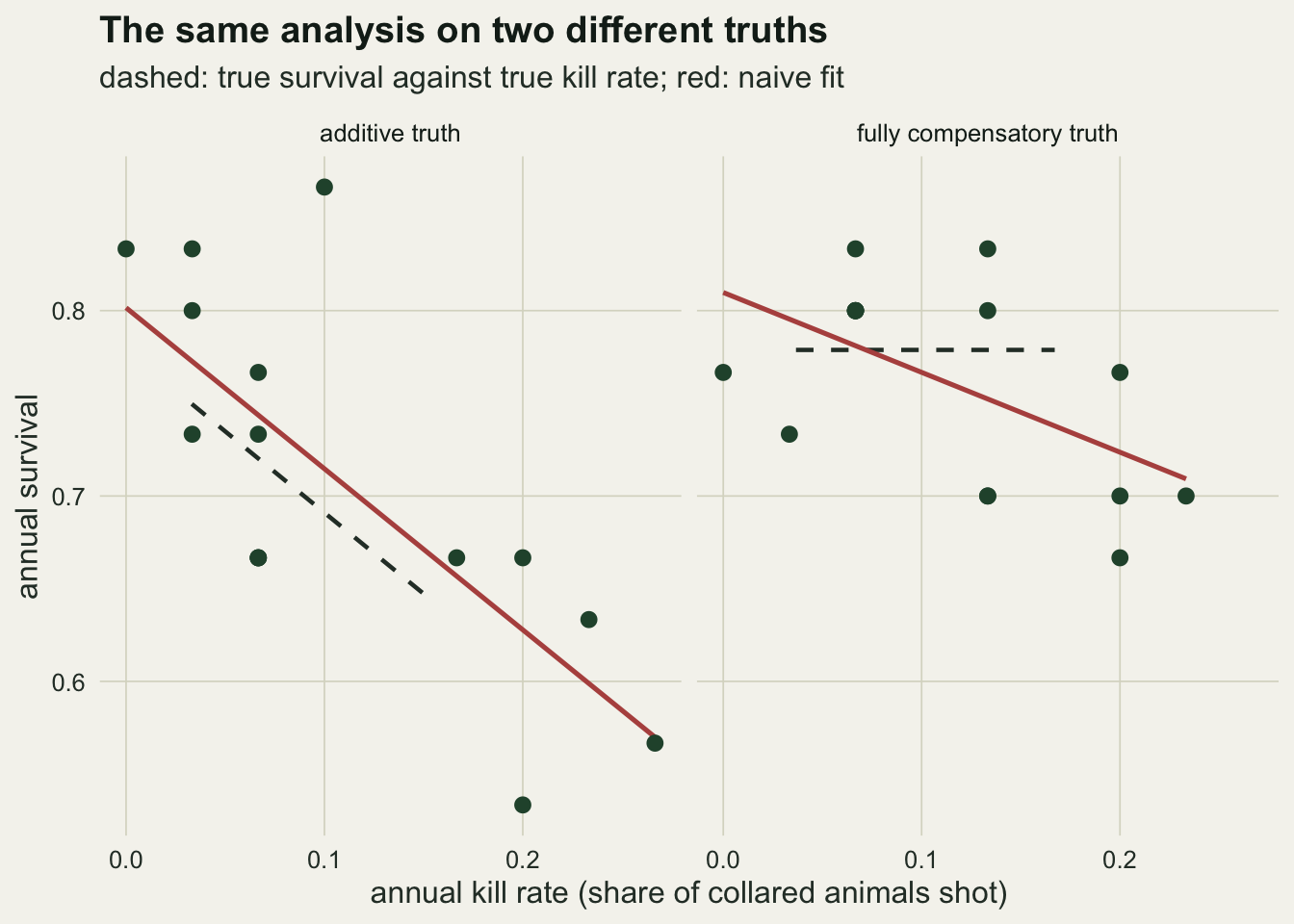
Shared fates put a covariance into both axes
In a year with true survival pS and true kill probability pK, the survivor share and the kill share of n animals are two cells of one multinomial count. Their sampling variances are pS (1 - pS) / n and pK (1 - pK) / n, and their sampling covariance is -pS pK / n, negative because an animal counted in one cell cannot be counted in the other.
set.seed(2211)
n_draw   <- 200000
p_one    <- fate_probs(0.11, "compensatory")
s_draw   <- rbinom(n_draw, n_small, p_one$s)
k_draw   <- rbinom(n_draw, n_small - s_draw, p_one$k / (1 - p_one$s))
cov_emp  <- cov(s_draw / n_small, k_draw / n_small)
cov_th   <- -p_one$s * p_one$k / n_small
var_emp  <- var(k_draw / n_small)
var_th   <- p_one$k * (1 - p_one$k) / n_small
cor_th   <- cov_th / sqrt(var_th * p_one$s * (1 - p_one$s) / n_small)
At a harvest hazard of 0.11 under compensation and 30 animals, 200000 simulated years give a covariance of -0.002523 against the formula’s -0.002527, and a variance of the kill share of 0.002920 against 0.002928. The sampling correlation between the two estimates is -0.616.
Across many years the least-squares slope converges to the covariance of the two estimated series divided by the variance of the estimated kill rate. Each of those is the between-year quantity plus the average sampling term, because the sampling errors of different years are independent. So with n animals a year and a long series, the naive slope tends to
slope = (Cov(pS, pK) - E[pS pK] / n) / (Var(pK) + E[pK (1 - pK)] / n)
where the covariance, variance and expectations are taken over years, and b = -slope / (E[pS] - slope E[pK]). Two artefacts sit in that formula. The term in the denominator is ordinary sampling noise in the predictor and pulls the slope towards zero, as in the regression dilution post. The term in the numerator is the shared-fates covariance and pushes the slope negative, towards additivity. Under additivity they partly offset each other. Under compensation Cov(pS, pK) is zero, there is no real slope for the dilution term to shrink, and only the push towards additivity is left. With survival constant, the formula collapses to
b = E[pK] / (E[pK] + (n - 1) Var(pK))
which does not involve survival at all: the bias is the mean kill rate set against n - 1 times the between-year variance of the kill rate.
b_formula <- function(truth, n_anim, lo = h_lo, hi = h_hi) {
  mm  <- pop_moments(truth, lo, hi)
  v_k <- mm$ekk - mm$ek^2
  c_k <- mm$esk - mm$es * mm$ek
  sl  <- (c_k - mm$esk / n_anim) / (v_k + (mm$ek - mm$ekk) / n_anim)
  -sl / (mm$es - sl * mm$ek)
}
n_set  <- c(30, 100, 400)
cf_add <- sapply(n_set, function(n) b_formula("additive", n))
cf_cmp <- sapply(n_set, function(n) b_formula("compensatory", n))

mom_cmp  <- pop_moments("compensatory")
ek_cmp   <- mom_cmp$ek
vk_cmp   <- mom_cmp$ekk - mom_cmp$ek^2
b_simple <- ek_cmp / (ek_cmp + (n_set - 1) * vk_cmp)
stopifnot(max(abs(b_simple - cf_cmp)) < 1e-8)
n_tenth  <- ceiling(1 + 9 * ek_cmp / vk_cmp)
cf_narrow <- b_formula("compensatory", n_small, 0.05, 0.15)
With the design above, the long-series naive b under compensation is 0.614, 0.317 and 0.103 for 30, 100 and 400 animals a year, where the truth is zero; the simplified form agrees with the general one to eight decimal places. Under additivity it is 1.047, 1.084 and 1.112, against a noiseless 1.125. Pushing the compensatory bias below 0.1 needs (n - 1) Var(pK) to exceed nine times E[pK], which here means at least 416 collared animals every year. The between-year spread of the kill rate is what buys the study its protection: if the harvest hazard only varies between 0.05 and 0.15, the long-series b under compensation at 30 animals rises to 0.824.
t_long <- 4000
r_long <- 500
set.seed(2212)
long_tab <- do.call(rbind, lapply(c("additive", "compensatory"), function(tr)
  do.call(rbind, lapply(n_set, function(n) {
    bb <- sim_studies(n, t_long, r_long, tr)$b
    data.frame(truth = tr, n_anim = n, b_mean = mean(bb), b_se = sd(bb) / sqrt(r_long))
  }))))
long_tab$formula <- ifelse(long_tab$truth == "additive", cf_add[match(long_tab$n_anim, n_set)],
                           cf_cmp[match(long_tab$n_anim, n_set)])
long_tab$z_gap <- (long_tab$b_mean - long_tab$formula) / long_tab$b_se
long_gap <- max(abs(long_tab$b_mean - long_tab$formula))
long_z   <- max(abs(long_tab$z_gap))
The formula is a limit, so it is checked against studies long enough to reach it: 500 simulated studies of 4000 years for each hypothesis and each number of animals. The mean simulated b differs from the formula by at most 0.0010, and by at most 1.8 Monte Carlo standard errors. The formula is reproduced; nothing in it is a simulation finding.
n_curve <- round(10^seq(log10(5), log10(2000), length.out = 60))
curve_df <- rbind(
  data.frame(n_anim = n_curve, truth = "additive", range = "0.02 to 0.20",
             b = sapply(n_curve, function(n) b_formula("additive", n))),
  data.frame(n_anim = n_curve, truth = "compensatory", range = "0.02 to 0.20",
             b = ek_cmp / (ek_cmp + (n_curve - 1) * vk_cmp)),
  data.frame(n_anim = n_curve, truth = "compensatory", range = "0.05 to 0.15",
             b = sapply(n_curve, function(n) b_formula("compensatory", n, 0.05, 0.15))))
curve_df$grp <- paste(curve_df$truth, curve_df$range)
ref_b <- data.frame(truth = c("additive", "compensatory"), b = c(b_pop, 0))
ggplot(curve_df, aes(n_anim, b, colour = truth)) +
  geom_hline(data = ref_b, aes(yintercept = b, colour = truth), linetype = "dashed",
             linewidth = 0.5, show.legend = FALSE) +
  geom_line(aes(group = grp, linetype = range), linewidth = 0.9) +
  geom_point(data = long_tab, aes(n_anim, b_mean), size = 2.8) +
  scale_x_log10(breaks = c(5, 10, 30, 100, 400, 2000)) +
  scale_colour_manual(values = c(additive = te_gold, compensatory = te_forest), name = "truth") +
  scale_linetype_manual(values = c("0.02 to 0.20" = "solid", "0.05 to 0.15" = "dotted"),
                        name = "harvest hazard") +
  labs(x = "animals collared each year (log scale)", y = "long-series naive b",
       title = "The bias is a formula in n and the spread of kill rates") +
  theme_datasheet() +
  theme(legend.position = "bottom", legend.box = "vertical")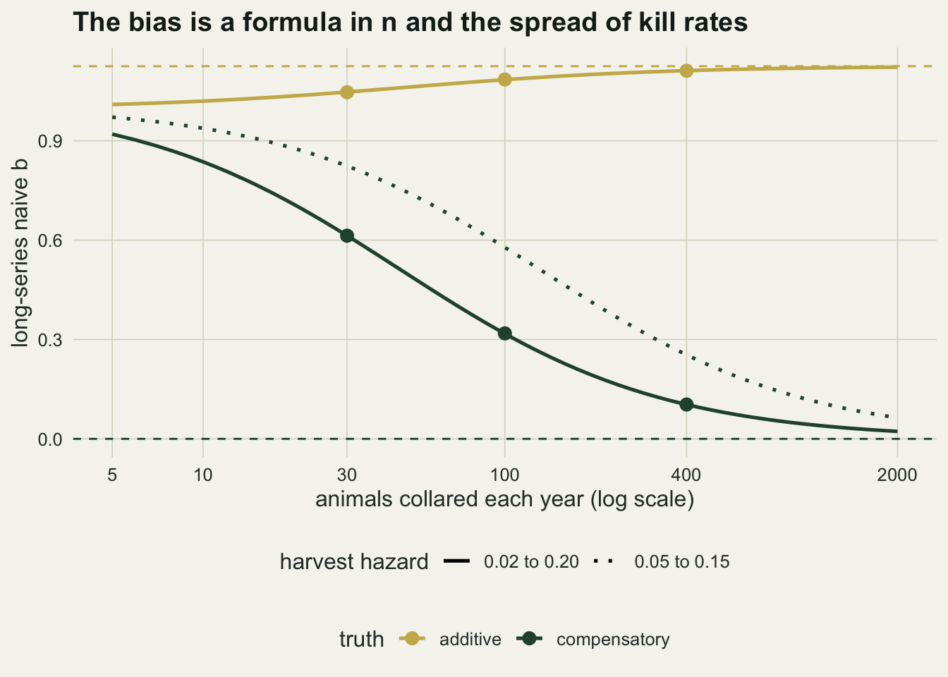
A longer series makes the false signal more certain
The analyst does not have four thousand years. The quantity that matters in practice is how often the naive test declares additivity when compensation is complete. Here that test is a one-sided t test of a negative slope at the 5 per cent level, decided before running: a rejection is read as evidence for additive mortality. Under compensation every rejection is a false one. Under additivity the same rejection rate is the power of the test, a different quantity.
The shared-fates covariance does not shrink as years are added. It is the average sampling covariance of one year, and averaging over more years estimates it more precisely rather than removing it. The standard error of the slope does shrink with more years. So the bias stays and the test becomes more sure of it.
t_set <- c(10, 15, 20, 30, 50)
r_rep <- 20000
set.seed(2213)
grid_runs <- list()
rate_tab  <- do.call(rbind, lapply(c("compensatory", "additive"), function(tr)
  do.call(rbind, lapply(n_set, function(n) do.call(rbind, lapply(t_set, function(ty) {
    sim <- sim_studies(n, ty, r_rep, tr)
    if (n == n_small && ty == t_small) grid_runs[[tr]] <<- sim
    rej <- mean(sim$t_val < qt(0.05, ty - 2))
    data.frame(truth = tr, n_anim = n, n_year = ty, rej = rej,
               rej_se = sqrt(rej * (1 - rej) / r_rep), b_med = median(sim$b),
               rej_two = mean(sim$t_val < qt(0.025, ty - 2)))
  }))))))
mc_se_max <- sqrt(0.25 / r_rep)

rt <- function(tr, n, ty, v = "rej") rate_tab[rate_tab$truth == tr & rate_tab$n_anim == n &
                                               rate_tab$n_year == ty, v]
false_head <- rt("compensatory", n_small, t_small)
false_se   <- rt("compensatory", n_small, t_small, "rej_se")
false_z    <- (false_head - 0.05) / false_se
stopifnot(false_z > 1)
false_two <- rt("compensatory", n_small, t_small, "rej_two")
pow_ratio <- rt("additive", n_small, t_small) / false_head

set.seed(2214)
ctrl_rej <- sapply(c(t_small, 50), function(ty) {
  sim <- sim_studies(n_small, ty, r_rep, "compensatory", split = TRUE)
  mean(sim$t_val < qt(0.05, ty - 2))
})
ctrl_se <- sqrt(ctrl_rej * (1 - ctrl_rej) / r_rep)
ctrl_add <- median(sim_studies(n_small, t_small, r_rep, "additive", split = TRUE)$b)

sd_set <- c(0.05, 0.10)
set.seed(2216)
noise_tab <- do.call(rbind, lapply(c("compensatory", "additive"), function(tr)
  do.call(rbind, lapply(sd_set, function(sdn) {
    sim <- sim_studies(n_small, t_small, r_rep, tr, sd_nat = sdn)
    data.frame(truth = tr, sd_nat = sdn, rej = mean(sim$t_val < qt(0.05, t_small - 2)),
               b_med = median(sim$b))
  }))))
nz <- function(tr, sdn, v) noise_tab[noise_tab$truth == tr & noise_tab$sd_nat == sdn, v]
cmp_med <- range(rate_tab$b_med[rate_tab$truth == "compensatory" & rate_tab$n_anim == n_small])
Each cell of the grid is 20000 simulated studies, fixed before running so that the Monte Carlo standard error of any rate is at most 0.0035.
With 30 animals a year for 15 years and fully compensatory harvest, the naive test declares additive mortality in 56.9 per cent of studies (Monte Carlo standard error 0.4 percentage points), against the nominal 5 per cent. Read as a two-sided test at 5 per cent, which rejects for a negative slope only below the 2.5 per cent quantile, the rate is 44.0 per cent, against a nominal 2.5 per cent for a negative verdict; this is the reading of the p value that summary(lm()) prints. Over 10 to 50 years the median naive b at that sample size stays between 0.602 and 0.611, while the false rate climbs from 41.7 per cent at 10 years to 83.7 per cent at 30 and 96.6 per cent at 50. More animals lower the bias and with it the rate, but do not stop the climb: with 400 animals a year the false rate is 12.5 per cent at 10 years and 37.2 per cent at 50.
The control removes the shared fates and nothing else. If the kill rate of each year is estimated from a second, independent group of 30 animals, the same test on the same compensatory truth rejects in 5.3 per cent of studies at 15 years and 4.9 per cent at 50 (standard errors 0.2 and 0.2 points). Sampling noise in both axes, curvature and the competing risk are all still there. The excess comes from the covariance. The control is not free: under additivity the independent kill rate is a noisy predictor with nothing to offset its dilution, and the median b of the control design at 15 years falls to 0.468.
Under additivity the power of the same test at 30 animals is 60.7 per cent at 10 years, 78.5 per cent at 15 and 97.5 per cent at 30. At 15 years that is 78.5 per cent of additive studies rejecting against 56.9 per cent of compensatory ones, a ratio of 1.38. A rejection is only moderately more likely under additivity than under full compensation.
Real natural mortality also varies from year to year for reasons unrelated to harvest. Adding a normal deviation with a standard deviation of 0.05 or 0.10 to each year’s natural hazard (truncated at zero), independent of the harvest hazard, lowers the false additive rate at 30 animals and 15 years to 46.9 and 34.3 per cent, and the power to 71.0 and 51.4 per cent. The median naive b under compensation stays at 0.593 and 0.586: the extra scatter widens the standard error, and the bias is still there.
rate_tab$panel <- factor(rate_tab$truth, c("compensatory", "additive"),
                         c("compensatory truth: false additive rate",
                           "additive truth: power"))
rate_tab$animals <- factor(sprintf("%d animals a year", rate_tab$n_anim),
                           sprintf("%d animals a year", n_set))
ctrl_df <- data.frame(n_year = c(t_small, 50), rej = ctrl_rej,
                      panel = factor(levels(rate_tab$panel)[1], levels(rate_tab$panel)))
ref_df  <- data.frame(panel = factor(levels(rate_tab$panel)[1], levels(rate_tab$panel)),
                      y = 0.05)
ggplot(rate_tab, aes(n_year, rej, colour = animals)) +
  geom_hline(data = ref_df, aes(yintercept = y), linetype = "dashed",
             colour = te_body, linewidth = 0.6) +
  geom_line(linewidth = 0.9) +
  geom_point(size = 2.2) +
  geom_point(data = ctrl_df, aes(n_year, rej), inherit.aes = FALSE,
             shape = 0, size = 3, stroke = 1, colour = te_ink) +
  facet_wrap(~ panel, ncol = 1) +
  scale_colour_manual(values = c(te_rust, te_gold, te_forest), name = NULL) +
  scale_y_continuous(limits = c(0, 1)) +
  scale_x_continuous(breaks = t_set) +
  labs(x = "years in the series", y = "share of studies rejecting",
       title = "More years, more false additivity") +
  theme_datasheet() +
  theme(legend.position = "bottom")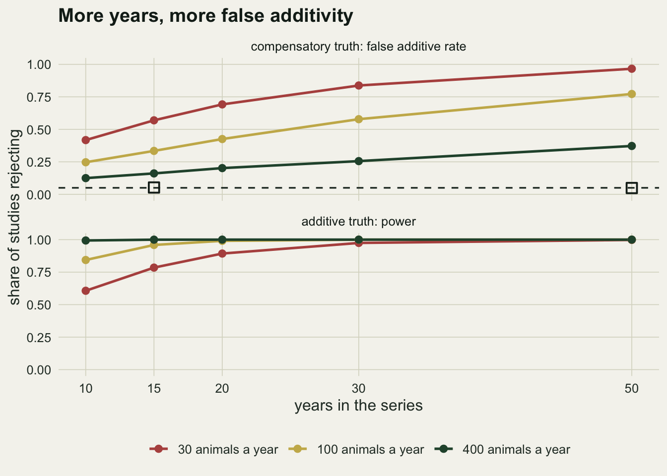
Subtracting the known sampling covariance
Because the sampling variance and covariance of a multinomial are known functions of the cell probabilities, they can be estimated in each year and subtracted, which is the method-of-moments correction for known error covariance set out by Fuller (1987). The corrected slope is the sample covariance of the two series minus the average estimated sampling covariance, divided by the sample variance of the kill rate minus its average estimated sampling variance. The plug-ins are -S K / (n - 1) for the covariance and K (1 - K) / (n - 1) for the variance, with the divisor n - 1 rather than n because that makes each plug-in unbiased for its multinomial target. When the corrected denominator is zero or negative the between-year spread of the kill rate is not distinguishable from sampling noise, and the estimate is undefined.
mom_sum <- function(sim) {
  ok <- !is.na(sim$b_c)
  c(defined = mean(ok),
    med = median(sim$b_c[ok]),
    q25 = unname(quantile(sim$b_c[ok], 0.25)), q75 = unname(quantile(sim$b_c[ok], 0.75)),
    naive_q25 = unname(quantile(sim$b, 0.25)), naive_q75 = unname(quantile(sim$b, 0.75)),
    naive_high = mean(sim$b > 0.5), corr_high = mean(sim$b_c[ok] > 0.5))
}
ms_cmp <- mom_sum(grid_runs[["compensatory"]])
ms_add <- mom_sum(grid_runs[["additive"]])

set.seed(2215)
r_mom <- 20000
mom_long <- t(sapply(t_set, function(ty) mom_sum(sim_studies(n_small, ty, r_mom, "compensatory"))))
mom_long_hi <- mom_sum(sim_studies(n_set[2], t_small, r_mom, "compensatory"))
bench_cmp <- median(grid_runs[["compensatory"]]$b_bench)
bench_add <- median(grid_runs[["additive"]]$b_bench)
At 30 animals and 15 years under full compensation, the correction is undefined in 9.7 per cent of studies. Where it is defined, its median b is 0.044, against a naive median of 0.602, so the bias is largely gone. The spread is the price: the 25th and 75th percentiles of the corrected b over studies are -0.83 and 0.53, where the naive b has 0.40 and 0.78. Under additivity the corrected median is 1.127, close to the noiseless 1.125, with a quartile range from 0.51 to 1.75, and it is undefined in 12.7 per cent of studies.
A simple way to read the cost is to ask which hypothesis each estimate sits nearer to, that is, whether b is above one half. Under compensation the naive b is above one half in 64.3 per cent of studies and the corrected b, where defined, in 26.7 per cent. Under additivity the shares are 92.1 and 75.2 per cent. The naive estimate puts 64.3 per cent of compensatory studies on the wrong side and 7.9 per cent of additive ones; the corrected estimate puts 26.7 and 24.8 per cent there. It trades one large error for two moderate ones, and on top of that it gives no answer at all in the studies where it is undefined.
Unlike the naive estimate, the corrected one improves with years. Under compensation at 30 animals, with 20000 studies per series length, its quartile range narrows from -0.87 to 0.64 at 10 years to -0.51 to 0.28 at 50, and the share of studies with no defined estimate falls from 16.5 to 0.4 per cent. With 100 animals and 15 years the quartile range is -0.36 to 0.21.
box_df <- do.call(rbind, lapply(c("compensatory", "additive"), function(tr) {
  sim <- grid_runs[[tr]]
  rbind(data.frame(truth = tr, method = "naive", b = sim$b),
        data.frame(truth = tr, method = "moment corrected", b = sim$b_c[!is.na(sim$b_c)]))
}))
box_df$truth  <- factor(box_df$truth, c("compensatory", "additive"),
                        c("compensatory truth (b = 0)", "additive truth"))
box_df$method <- factor(box_df$method, c("naive", "moment corrected"))
out_view <- mean(box_df$b[box_df$method == "moment corrected"] < -2 |
                 box_df$b[box_df$method == "moment corrected"] > 3)
truth_df <- data.frame(truth = levels(box_df$truth), b = c(0, b_pop))
truth_df$truth <- factor(truth_df$truth, levels(box_df$truth))
ggplot(box_df, aes(method, b, fill = method)) +
  geom_hline(data = truth_df, aes(yintercept = b), linetype = "dashed",
             colour = te_body, linewidth = 0.6) +
  geom_boxplot(outlier.shape = NA, width = 0.5, colour = te_ink, linewidth = 0.5) +
  facet_wrap(~ truth) +
  coord_cartesian(ylim = c(-2, 3)) +
  scale_fill_manual(values = c(te_rust, te_forest), guide = "none") +
  labs(x = NULL, y = "estimated b",
       title = "The correction removes the bias and keeps the noise",
       subtitle = "dashed: the noiseless b of each truth") +
  theme_datasheet()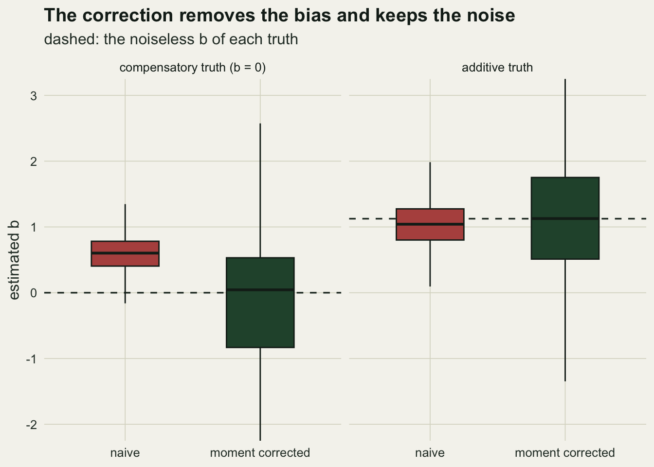
Across both hypotheses, 14.4 per cent of the defined corrected estimates fall outside the window drawn in the figure.
What to report
Report where the survival and the kill rate come from. If both are shares of the same marked animals, the regression of one on the other is not a test of compensation, and saying so is the first line of any analysis that uses it. The formula above gives the size of the problem from three quantities the analyst has: the number of animals a year, the mean kill rate and the between-year variance of the kill rate. Under full compensation the naive b tends to E[pK] / (E[pK] + (n - 1) Var(pK)). Because the observed variance of the kill rates already contains the sampling variance, the same limit can be written with observed quantities only, as mean(K) / (n var(K) + mean(K)^2), and that benchmark belongs next to the fitted b. Over the simulated studies of 30 animals and 15 years its median is 0.637 under compensation and 0.674 under additivity, against naive medians of 0.602 and 1.041: a fitted b near the benchmark is what full compensation looks like through this design.
Do not read a significant negative slope from a long series as stronger evidence than one from a short series. In this design the false additive rate at 30 animals rose from 41.7 to 96.6 per cent between 10 and 50 years, because what the extra years estimate more precisely is the bias.
If the correction is used, report how often it is defined, report the moment-corrected b with an interval (a parametric bootstrap from the fitted multinomial is one candidate; it was not tested here), and expect that interval to be wide. The correction here was not paired with a test. At 30 animals and 15 years the middle half of its estimates runs from -0.83 to 0.53 under compensation and from 0.51 to 1.75 under additivity, so the two middle halves meet near one half. A design with independent sources for the two rates, such as a kill rate from a separate marked sample, removes the covariance at the source, as the control above did; it dilutes a real slope instead, as the control’s additive median of 0.468 showed.
Keep the noiseless value in view. Even with perfect data, additive hazards acting together through the year give b = 1.125 over this design, not one; the value depends on the natural hazard and on when in the year the harvest falls, from 1.000 for a season before any natural mortality to 1.284 for one after all of it. A fitted b somewhat above one is what full additivity can look like, not evidence of mortality beyond additive.
Honest limits
Only known-fate telemetry was simulated, with every animal’s fate observed and the same number of animals every year. Band-recovery designs estimate survival and the recovery or kill rate from a different likelihood, with a different sampling covariance that includes the reporting rate; nothing above measures them.
The compensatory truth is full and linear: the natural hazard falls one for one with the harvest hazard, and total mortality never changes. Real compensation may be partial or may stop above a threshold, as in the threshold hypothesis of the adaptive management post. Year-to-year variation in natural mortality was tried only as normal noise on the hazard, independent of harvest, at one sample size and one series length; variation that is correlated with harvest, for example through weather that shortens a season and kills animals in the same winter, would enter the slope directly and was not simulated. Every simulated year has the two hazards acting together. A season that falls before or after most natural mortality changes the additive b, as the two closed-form extremes of the first section show, and with it the power of the test, which was measured for concurrent hazards only. Under full compensation survival is constant whatever the timing, so the long-series formula keeps its form; only the mean and the variance of the kill rate that enter it change.
The harvest hazards were drawn independently and uniformly each year. A kill rate that drifts over time, or that follows population size, would add a confounded trend to both axes that this simulation does not contain.
The moment correction was measured as an estimator only. Its sampling distribution is skewed and it is sometimes undefined, so a normal-theory interval would be a poor guide; a parametric bootstrap from the fitted multinomial would be the next thing to try, and it was not tried here. Fuller (1987) also gives a modified version of the moment estimator that stays defined when the corrected denominator is small or negative; it was not tried either. Likelihood approaches that model the fates directly and estimate the process correlation, such as the state-space model of Servanty and colleagues (2010), were not simulated either, and Peron (2013) reviews the wider set of methods and their sources of bias.
The one-sided test at 5 per cent is one choice, and the two-sided reading quoted above already gives a different rate. A test of b = 1 against b = 0, or a comparison of AIC between the two regression forms, would give different rates again, and neither was simulated; both are built on the same biased slope.
References
Burnham KP, Anderson DR 1984 Ecology 65(1):105-112 (10.2307/1939463)
Lebreton JD 2005 Australian and New Zealand Journal of Statistics 47(1):49-63 (10.1111/j.1467-842X.2005.00371.x)
Servanty S, Choquet R, Baubet E, Brandt S, Gaillard JM, Schaub M, Toigo C, Lebreton JD, Buoro M, Gimenez O 2010 Ecology 91(7):1916-1923 (10.1890/09-1931.1)
Peron G 2013 Journal of Animal Ecology 82(2):408-417 (10.1111/1365-2656.12014)
Fuller WA 1987 Measurement Error Models (ISBN 978-0-471-86187-4)