library(ggplot2)

te_paper  <- "#f5f4ee"
te_ink    <- "#16241d"
te_body   <- "#2c3a31"
te_forest <- "#275139"
te_rust   <- "#b5534e"
te_gold   <- "#c9b458"
te_line   <- "#dad9ca"

theme_datasheet <- function() {
  theme_minimal(base_size = 12) +
    theme(plot.background  = element_rect(fill = te_paper, colour = NA),
          panel.background = element_rect(fill = te_paper, colour = NA),
          panel.grid.major = element_line(colour = te_line, linewidth = 0.3),
          panel.grid.minor = element_blank(),
          text             = element_text(colour = te_body),
          plot.title       = element_text(colour = te_ink, face = "bold"),
          plot.subtitle    = element_text(colour = te_body),
          axis.text        = element_text(colour = te_body))
}Reconstructing a population from ages at harvest
R
population dynamics
harvest
wildlife management
fisheries
likelihood
simulation
ecology tutorial
Ages at harvest alone leave the harvest rate on an exact ridge, so abundance is a guess. Cohort analysis, the flat profile and what known effort buys, in R.
A wildlife agency runs compulsory check stations for white-tailed deer. Every deer shot in the district is brought in, a technician pulls a tooth or reads the wear on the jaw, and the animal goes into a table by year and by age. After twelve seasons the table holds several thousand aged carcasses, and the question put to it is always the same one: how many deer are out there this year, and is the harvest taking too many of them? The same table exists for black bear, elk, moose and fisher, and in fisheries it is the catch at age, which has been turned into abundance since Fry (1949) summed the catches of each year class into a virtual population.
The attraction is that a harvested animal is a certain record. It was alive in the year it was shot, at the age it was aged, and every other member of its cohort that was shot later was alive in all the years between. Add up a cohort’s harvest diagonally through the table and you have a floor under that cohort’s size. What the table does not say is how much of the cohort was never shot, and that single missing number, the harvest rate, turns out to decide almost everything a manager wants from the reconstruction.
This post demonstrates a known result rather than a new one. Statistical population reconstruction writes the age-at-harvest table as a likelihood with cohort sizes, survival and harvest probability as parameters, as Gove and colleagues (2002) set out. Bellier and colleagues (2024) note that this frequentist line of work requires auxiliary data, radio-telemetry for instance, and built a Bayesian hierarchical model that reconstructs the population without it; they report that their simulations recover abundance and rates well once the table has more than two age classes, and that the prior information placed on the demographic rates affects the accuracy of the estimates. Their model differs from the one here in the ways listed under Honest limits. The measurements below show why the prior matters, in the simplest version of the model: at constant effort the ages identify only two products of the parameters, so the harvest rate sits on an exact ridge, and whatever a fit reports for it comes from the starting point, the prior or the way the cohort sizes are handled.
Nothing here repeats what the fisheries posts already cover. Stock-recruitment and reference points ends with catch curves, including one year class followed across years, and those return a mortality rate from the slope of log catch at age; the intercept that would carry abundance is exactly the part a catch curve throws away. Borrowed age-length keys and strong year classes is about where the ages come from in the first place, when only some fish are aged, and it too closes on a catch curve. Checking a stock assessment works on a surplus production model with no ages in it; its check on contrast is the same idea as the effort contrast below, for growth rate and carrying capacity instead of harvest rate, and its catchability that creeps upward a few per cent a year returns at the end of this post. The one-way trip in surplus production models in R is the closest cousin of the ridge: a series that only ever declines pins down something close to a product of growth rate and carrying capacity, and the two trade off along a ridge; in the age table below, the product is exact.
A harvested population and its table
The simulated population has six age classes and is followed for twelve years. Each year a new cohort of yearlings enters, with a mean of a thousand animals and lognormal year-to-year variation. The harvest comes first: every animal alive at the start of the season is shot with probability h, the same at every age. The survivors then live to the next year with natural survival s. Harvest probability is tied to hunting effort E by h = 1 - exp(-c E), the chance that an animal meets at least one hunter when encounters occur at rate c per unit effort. Effort is scaled to average one, so c fixes the harvest rate in an average year. Animals that reach the oldest class leave the table after that year; there is no plus group.
n_year   <- 12
n_age    <- 6
s_true   <- 0.8
c_true   <- 0.25
rec_mean <- 1000
rec_sd   <- 0.3
h_true   <- 1 - exp(-c_true)

cell_year   <- rep(seq_len(n_year), times = n_age)
cell_age    <- rep(seq_len(n_age), each = n_year)
cell_cohort <- cell_year - cell_age + n_age
cell_entry  <- pmax(1, cell_year - cell_age + 1)
cell_k      <- cell_year - cell_entry
n_cohort    <- n_year + n_age - 1

sim_harvest <- function(effort, s = s_true, cc = c_true) {
  h_year <- 1 - exp(-cc * effort)
  n_mat  <- matrix(0, n_year, n_age)
  h_mat  <- matrix(0, n_year, n_age)
  n_mat[1, ] <- round(rec_mean * (s * exp(-cc))^(0:(n_age - 1)))
  for (yr in seq_len(n_year)) {
    if (yr > 1) {
      n_mat[yr, 1] <- rpois(1, rec_mean * exp(rnorm(1, 0, rec_sd)))
      alive <- n_mat[yr - 1, -n_age] - h_mat[yr - 1, -n_age]
      n_mat[yr, -1] <- rbinom(n_age - 1, alive, s)
    }
    h_mat[yr, ] <- rbinom(n_age, n_mat[yr, ], h_year[yr])
  }
  list(abund = n_mat, harvest = h_mat, h_year = h_year)
}

effort_flat <- rep(1, n_year)
set.seed(4417)
herd <- sim_harvest(effort_flat)
herd_total  <- sum(herd$harvest)
herd_last_n <- sum(herd$abund[n_year, ])
herd_last_c <- sum(herd$harvest[n_year, ])
All of these values were fixed before any fitting was run. Natural survival is 0.8 and c is 0.25, a harvest probability of 0.221 in a year of average effort, which is a moderately hunted deer herd. One run at constant effort gives the table below: 6392 aged animals over the twelve years, 549 of them in the final season, taken from a population of 2373 alive at the start of that season. A cohort runs down a diagonal: the yearlings of one year are the two year olds of the next.
tab_df <- data.frame(year = cell_year, age = cell_age,
                     n_shot = as.vector(herd$harvest))
one_cohort <- tab_df[cell_cohort == 8, ]

ggplot(tab_df, aes(year, age)) +
  geom_tile(aes(fill = n_shot), colour = te_paper, linewidth = 0.6) +
  geom_tile(data = one_cohort, fill = NA, colour = te_rust, linewidth = 1.1) +
  geom_text(aes(label = n_shot,
                colour = n_shot > 0.55 * max(n_shot)), size = 3.2,
            show.legend = FALSE) +
  scale_fill_gradient(low = te_line, high = te_forest, name = "animals shot") +
  scale_colour_manual(values = c(`FALSE` = te_ink, `TRUE` = te_paper)) +
  scale_x_continuous(breaks = seq_len(n_year), expand = c(0, 0)) +
  scale_y_continuous(breaks = seq_len(n_age), expand = c(0, 0)) +
  labs(x = "year", y = "age class",
       title = "The age-at-harvest table",
       subtitle = "outlined in red: the yearlings of year 3 followed to age 6") +
  theme_datasheet() +
  theme(panel.grid.major = element_blank(), legend.position = "right")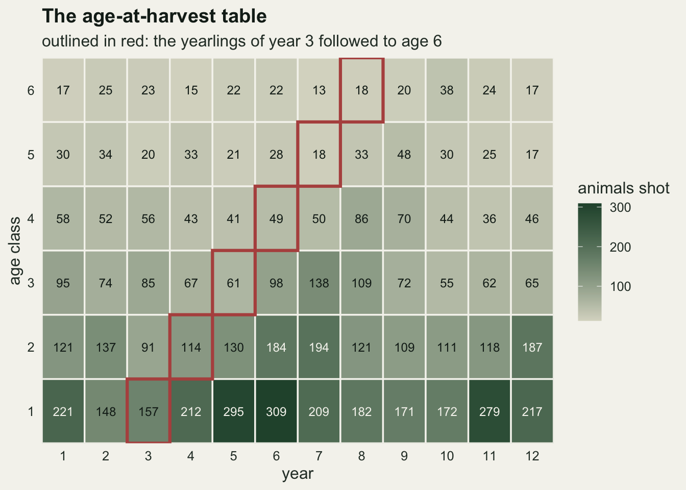
Backward cohort analysis: the last year is the guess
The oldest reconstruction method needs no likelihood. Take natural survival as known, and start from the last cell of each cohort, where the cohort leaves the table either because the series ends or because it has reached the oldest class. The cohort size in that cell is its harvest divided by the harvest rate, which has to be supplied. From there the cohort is walked backwards one year at a time: the number alive a year earlier is the number alive now divided by s, plus the animals shot in that earlier year. That is virtual population analysis in its simplest form, with survival known and harvest applied as a pulse.
The consequence for the final year can be written down before simulating anything. Every cell in the final year is a terminal cell, so the reconstructed population in the final year is the final harvest divided by the guessed rate. Divided by the same harvest over the true rate, the ratio is h / h_guess exactly: a guess of half the true rate doubles the estimate, a guess half again too high cuts it to two thirds. The simulation reproduces this closed form; it is not a finding.
cohort_back <- function(harvest, h_guess, s = s_true) {
  n_hat <- matrix(NA_real_, n_year, n_age)
  n_hat[n_year, ] <- harvest[n_year, ] / h_guess
  n_hat[, n_age]  <- harvest[, n_age] / h_guess
  for (yr in (n_year - 1):1) for (ag in (n_age - 1):1)
    n_hat[yr, ag] <- n_hat[yr + 1, ag + 1] / s + harvest[yr, ag]
  rowSums(n_hat)
}
guess_mult <- c(0.5, 1, 1.5)

vpa_exact <- vapply(guess_mult, function(gm)
  cohort_back(herd$harvest, gm * h_true)[n_year] /
    cohort_back(herd$harvest, h_true)[n_year], 0)
stopifnot(max(abs(vpa_exact - 1 / guess_mult)) < 1e-12)

# closed form for every year: relative error (h / h_guess - 1) (1 - h)^k,
# k = steps to the terminal cell, weighted by the expected age structure
u_w   <- (s_true * (1 - h_true))^(0:(n_age - 1))
steps <- sapply(seq_len(n_year), function(yr) pmin((n_age - 1):0, n_year - yr))
keep  <- colSums(u_w * (1 - h_true)^steps) / sum(u_w)
vpa_closed_yr <- 1 + outer(keep, 1 / guess_mult - 1)

n_rep_vpa <- 400
set.seed(5521)
vpa_sim <- replicate(n_rep_vpa, {
  d_sim <- sim_harvest(effort_flat)
  truth <- rowSums(d_sim$abund)
  vapply(guess_mult, function(gm)
    cohort_back(d_sim$harvest, gm * h_true) / truth, numeric(n_year))
})
vpa_med <- apply(vpa_sim, c(1, 2), median)
vpa_lo  <- apply(vpa_sim, c(1, 2), quantile, probs = 0.1)
vpa_hi  <- apply(vpa_sim, c(1, 2), quantile, probs = 0.9)
vpa_gap <- max(abs(vpa_med - vpa_closed_yr))
stopifnot(vpa_gap < 0.02)
On the table above the final-year ratio between the reconstructions is exactly the inverse of the guess multiplier (the chunk checks it). Over 400 simulated tables, the median ratio of the final-year estimate to the true final-year population is 2.00 for the low guess, 1.00 for the correct one and 0.67 for the high guess.
The early years are less exposed, and the reason is again arithmetic. Walking back a year divides the terminal error by s, but the cohort was larger a year earlier by 1 / ((1 - h) s), so relative to the cohort the error left by the guess shrinks by the escape probability 1 - h each year, not by survival: k years before its terminal cell a cohort carries a relative error of (h / h_guess - 1)(1 - h)^k. Every cohort alive in year one reaches its terminal cell at age six, zero to five years later, so the first-year ratio is one plus (h / h_guess - 1) times the mean of (1 - h)^k weighted by the expected age structure: 1.423 and 0.859 for the two wrong guesses, against simulated medians of 1.42 and 0.86. With k capped by the end of the series the same sum gives every year of the figure below, and the medians stay within 0.009 of it throughout. With h near 0.22 and at most five steps back, the first year still carries 0.423 of the final year’s relative error; the heavier the harvest, the faster the backward walk forgets the guess. The years a manager looks at least carry the least error, and the year that sets next season’s quota carries all of it.
vpa_df <- do.call(rbind, lapply(seq_along(guess_mult), function(i)
  data.frame(year = seq_len(n_year), med = vpa_med[, i],
             lo = vpa_lo[, i], hi = vpa_hi[, i], closed = vpa_closed_yr[, i],
             guess = sprintf("guessed rate %.1f x true", guess_mult[i]))))

ggplot(vpa_df, aes(year, med, colour = guess, fill = guess)) +
  geom_hline(yintercept = 1, linetype = "dashed", colour = te_body,
             linewidth = 0.5) +
  geom_ribbon(aes(ymin = lo, ymax = hi), alpha = 0.18, colour = NA) +
  geom_line(linewidth = 0.9) +
  geom_point(size = 1.8) +
  geom_point(aes(y = closed), shape = 4, size = 3, colour = te_ink,
             show.legend = FALSE) +
  scale_colour_manual(values = c(te_rust, te_ink, te_forest), name = NULL) +
  scale_fill_manual(values = c(te_rust, te_ink, te_forest), name = NULL) +
  scale_x_continuous(breaks = seq_len(n_year)) +
  labs(x = "year", y = "reconstructed / true population",
       title = "The error grows towards the present",
       subtitle = "crosses: the closed form; the final year returns the true rate over the guess") +
  theme_datasheet() +
  theme(legend.position = "bottom")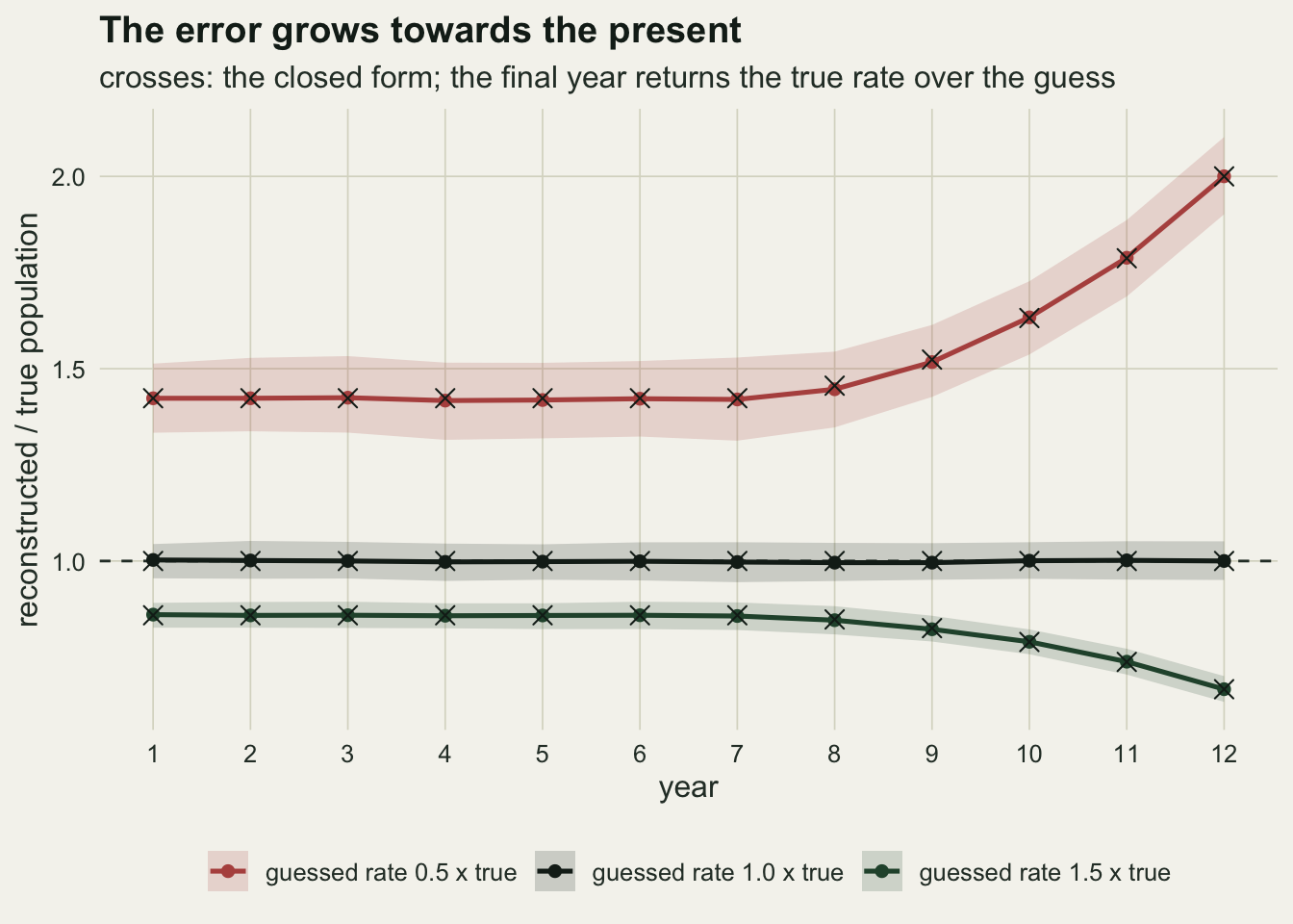
The likelihood without effort data has an exact ridge
Statistical reconstruction replaces the guessed rate with an estimated one. Each cohort j has a size R_j when it first appears in the table. An animal of that cohort is shot in its first year with probability h, and k years later with probability ((1 - h) s)^k h, having escaped the hunters and survived k times. The expected harvest in that cell is R_j times that probability. Each cell count is treated as Poisson with this mean, and for given s and c the cohort sizes have a closed-form maximum, the cohort’s total harvest divided by its summed cell probabilities, so the likelihood can be profiled down to two parameters.
Now hold effort constant. The expected harvest of cohort j in its k-th year is R_j h ((1 - h) s)^k. The data see R_j h and (1 - h) s and nothing else. Any other harvest rate h’ can be paired with a cohort size R_j h / h’ and a survival (1 - h) s / (1 - h’) that reproduce every expected count exactly, as long as that survival stays below one. The likelihood is therefore exactly flat along a curve in the (h, s) plane, and the final-year population, which is again the final harvest divided by h, moves along that curve freely.
cell_prob <- function(s, cc, effort) {
  h_year <- 1 - exp(-cc * effort)
  log_esc <- c(0, cumsum(-cc * effort))
  s^cell_k * exp(log_esc[cell_year] - log_esc[cell_entry]) * h_year[cell_year]
}
nll_age <- function(theta, harvest, effort) {
  p_cell <- cell_prob(plogis(theta[1]), exp(theta[2]), effort)
  y_cell <- as.vector(harvest)
  r_hat  <- rowsum(y_cell, cell_cohort)[, 1] / rowsum(p_cell, cell_cohort)[, 1]
  -sum(dpois(y_cell, r_hat[cell_cohort] * p_cell, log = TRUE))
}

u_ridge <- 0.6
h_on_ridge <- c(0.1, 0.2, 0.3)
nll_on_ridge <- vapply(h_on_ridge, function(hh)
  nll_age(c(qlogis(u_ridge / (1 - hh)), log(-log(1 - hh))),
          herd$harvest, effort_flat), 0)
ridge_spread <- diff(range(nll_on_ridge))

start_c <- c(0.05, 0.1, 0.2, 0.4, 0.8)
starts_fit <- t(vapply(start_c, function(sc) {
  o <- optim(c(qlogis(0.7), log(sc)), nll_age, harvest = herd$harvest,
             effort = effort_flat, control = list(maxit = 3000))
  h_est <- 1 - exp(-exp(o$par[2]))
  c(nll = o$value, h = h_est, s = plogis(o$par[1]),
    ratio = herd_last_c / h_est / herd_last_n)
}, numeric(4)))
start_nll_spread <- diff(range(starts_fit[, "nll"]))
u_fits <- (1 - starts_fit[, "h"]) * starts_fit[, "s"]
u_hat <- median(u_fits)
h_wall <- 1 - u_hat
The ridge is exact, not approximately flat. At three points with (1 - h) s = 0.6 and harvest rates of 0.1, 0.2 and 0.3, the negative log likelihood of the table above is 247.037301 each time, and the three are equal to within floating-point rounding.
A numerical optimiser has to stop somewhere on that curve, and where it stops depends on where it started. Five fits to the same table, started at c values from 0.05 to 0.8, reach negative log likelihoods within \(8.4 \times 10^{-6}\) of each other and harvest rates from 0.078 to 0.267. Their final-year populations run from 0.87 to 2.95 times the truth. Taking the best of several starts does not help: the best start is decided by optimiser tolerance, not by the data. None of these numbers is an estimate, and a single-start fit at constant effort that happens to land near the truth is the same accident as one that lands at twice it. What the fits do agree on is the product (1 - h) s, between 0.6182 and 0.6183, and that sets the only wall on the ridge: survival cannot exceed one, so no harvest rate above 0.382 fits.
Known effort bends the ridge into a bowl
If effort changes from year to year and the analyst knows by how much, the harvest rate is no longer one number. A heavy season takes a larger share of every cohort and leaves fewer of them for the next year, and a harvest probability that saturates as effort rises does not scale in proportion to effort. Both effects depend on c itself, not on c times a cohort size, so a table with varying effort carries information about c that a table at constant effort does not have. That information is a matter of Fisher information rather than of algebra: it grows with the contrast in effort, and there is no closed form for how much a given contrast buys.
make_effort <- function(sd_e, kind) {
  e_raw <- if (kind == "random") exp(rnorm(n_year, 0, sd_e)) else {
    g_lin <- seq(1, -1, length.out = n_year)
    exp(g_lin * sd_e / sd(g_lin))
  }
  e_raw / mean(e_raw)
}
set.seed(6630)
effort_var <- make_effort(0.5, "random")
herd_var   <- sim_harvest(effort_var)

h_grid <- seq(0.005, 0.55, by = 0.0025)
profile_h <- function(harvest, effort, nll_fun) {
  vapply(h_grid, function(hh) {
    lc <- log(-log(1 - hh))
    optimize(function(ls) nll_fun(c(ls, lc), harvest, effort), c(-6, 14))$objective
  }, 0)
}
prof_flat <- profile_h(herd$harvest, effort_flat, nll_age)
prof_var  <- profile_h(herd_var$harvest, effort_var, nll_age)
prof_flat <- prof_flat - min(prof_flat)
prof_var  <- prof_var - min(prof_var)

flat_zone  <- h_grid < h_wall - 0.01
flat_range <- max(prof_flat[flat_zone])
var_min_h  <- h_grid[which.min(prof_var)]
var_ci     <- range(h_grid[prof_var < qchisq(0.95, 1) / 2])
The profile over the harvest rate makes the difference visible. At constant effort the profile varies by at most \(2.3 \times 10^{-7}\) log-likelihood units everywhere below the survival wall at 0.382, which is optimiser tolerance; above the wall it climbs steeply, because survival would have to exceed one. With effort varying at a log standard deviation of 0.5 in a second simulated table, the profile has a minimum at 0.203 against a true 0.221, and the harvest rates within 1.92 log-likelihood units of it, an approximate 95 per cent interval, run from 0.108 to 0.288.
prof_df <- data.frame(h = h_grid, d_nll = c(prof_flat, prof_var), case = rep(
  c("constant effort", "effort known, log sd 0.5"), each = length(h_grid)))

ggplot(prof_df, aes(h, d_nll, colour = case)) +
  geom_vline(xintercept = h_true, linetype = "dashed", colour = te_body,
             linewidth = 0.5) +
  geom_hline(yintercept = qchisq(0.95, 1) / 2, linetype = "dotted",
             colour = te_body, linewidth = 0.5) +
  geom_line(linewidth = 1) +
  scale_colour_manual(values = c(te_rust, te_forest), name = NULL) +
  coord_cartesian(ylim = c(-0.25, 12), expand = FALSE) +
  labs(x = "harvest probability in an average year",
       y = "profile negative log likelihood (above minimum)",
       title = "A flat ridge, and a bowl once effort varies",
       subtitle = "dotted: 1.92 units, the usual 95 per cent cut; axis cut at 12") +
  theme_datasheet() +
  theme(legend.position = "bottom")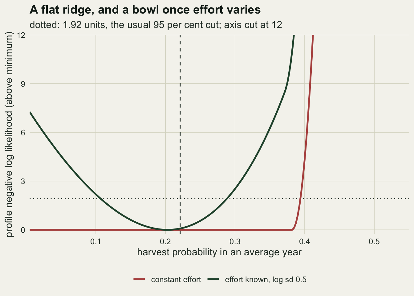
A prior on the harvest rate comes back unchanged
A Bayesian version of the same model is identified at constant effort, in the sense that it returns a posterior, but the posterior of the harvest rate can only be what the prior put there. The chunk below makes that concrete. Two analysts put different beta priors on the harvest rate in an average year, with means of 0.15 and 0.30, and each multiplies the prior by the profile likelihood above and normalises over the grid. At constant effort the profile is flat below the wall, so each posterior is its own prior cut off at the wall.
prior_ab <- list(low = c(3, 17), high = c(9, 21))
post_on_grid <- function(prof, ab) {
  w_prior <- dbeta(h_grid, ab[1], ab[2])
  w_post  <- w_prior * exp(-prof)
  list(prior = w_prior / sum(w_prior), post = w_post / sum(w_post))
}
grid_median <- function(w) h_grid[which(cumsum(w) >= 0.5)[1]]

post_tab <- do.call(rbind, lapply(names(prior_ab), function(nm) {
  pf <- post_on_grid(prof_flat, prior_ab[[nm]])
  pv <- post_on_grid(prof_var, prior_ab[[nm]])
  flat_ratio_w <- pf$post[flat_zone] / pf$prior[flat_zone]
  h_last_var <- function(hh) 1 - (1 - hh)^effort_var[n_year]
  data.frame(prior = nm, prior_med = grid_median(pf$prior),
             flat_med = grid_median(pf$post), var_med = grid_median(pv$post),
             flat_gap = diff(range(flat_ratio_w)) / mean(flat_ratio_w),
             above_wall = sum(pf$prior[h_grid >= h_wall]),
             flat_ratio = herd_last_c / grid_median(pf$post) / herd_last_n,
             var_ratio = sum(herd_var$harvest[n_year, ]) /
               h_last_var(grid_median(pv$post)) / sum(herd_var$abund[n_year, ]))
}))
stopifnot(max(post_tab$flat_gap) < 1e-5)
Below the wall each constant-effort posterior is its prior times a constant: across the grid the ratio of posterior to prior varies by at most \(2.3 \times 10^{-7}\) of its own size. The only thing the table removes is the part of the prior above the wall, 0.008 of the low prior’s mass and 0.162 of the high one’s, and that cut is all that separates posterior from prior: under the high prior the median moves from 0.295 to 0.280, and under the low prior from 0.138 to 0.138. The two analysts therefore report final-year populations of 1.68 and 0.83 times the truth from the same table, and each would be right to say the data were fitted well. On the table with varying effort the same two priors give posterior medians of 0.182 and 0.223, and final-year populations of 1.24 and 1.01 times the truth. Implicit information in integrated models shows a milder form of the same dependence: a rate with no data of its own is estimated through the model and absorbs whatever the model gets wrong. At constant effort the age-at-harvest table does not even offer that; beyond the survival wall it says nothing about the harvest rate at all.
What the cohort sizes add
The Poisson form above is not the only way to write the likelihood. Each animal of cohort j is shot in exactly one cell or never shot while it is in the table, so the cohort’s harvest is a multinomial draw of R_j animals over its cells plus a cell for the animals never taken. That is the exact likelihood of the simulator. It splits into two parts. Given the cohort’s total harvest, the spread of that harvest over the cells is multinomial with probabilities proportional to the cell probabilities, and that conditional part is exactly the profiled Poisson likelihood plus a constant. The other part is the cohort’s total, a single binomial draw from R_j animals with the cohort’s summed probability of being shot. With R_j unknown, one binomial draw cannot separate R_j from that probability, and when R_j is maximised out the fit always improves as that probability rises, towards the smallest population that could have produced the count.
nll_full <- function(theta, harvest, effort) {
  p_cell <- cell_prob(plogis(theta[1]), exp(theta[2]), effort)
  y_cell <- as.vector(harvest)
  s_tot  <- rowsum(y_cell, cell_cohort)[, 1]
  log_q  <- log(1 - rowsum(p_cell, cell_cohort)[, 1])
  score  <- function(x) digamma(x + s_tot + 1) - digamma(x + 1) + log_q
  lo_b <- rep(0, n_cohort)
  hi_b <- rep(log(1e9), n_cohort)
  for (i in 1:60) {
    mid_b <- (lo_b + hi_b) / 2
    up_b  <- score(expm1(mid_b)) > 0
    lo_b[up_b]  <- mid_b[up_b]
    hi_b[!up_b] <- mid_b[!up_b]
  }
  x_hat <- expm1((lo_b + hi_b) / 2)
  x_hat[score(0) <= 0] <- 0
  -sum(lgamma(x_hat + s_tot + 1) - lgamma(x_hat + 1) + x_hat * log_q) -
    sum(y_cell * log(p_cell)) + sum(lgamma(y_cell + 1))
}
cond_mult <- function(theta, harvest, effort) {
  p_cell <- cell_prob(plogis(theta[1]), exp(theta[2]), effort)
  y_cell <- as.vector(harvest)
  -sum(vapply(split(seq_along(y_cell), cell_cohort), function(ix)
    dmultinom(y_cell[ix], prob = p_cell[ix] / sum(p_cell[ix]), log = TRUE), 0))
}
set.seed(7102)
theta_try <- cbind(rnorm(4, 1, 0.5), rnorm(4, -1.3, 0.4))
pois_minus_cond <- apply(theta_try, 1, function(th)
  nll_age(th, herd$harvest, effort_flat) - cond_mult(th, herd$harvest, effort_flat))
cond_const_gap <- diff(range(pois_minus_cond))

prof_full <- profile_h(herd$harvest, effort_flat, nll_full)
prof_full <- prof_full - min(prof_full)
full_min_h <- h_grid[which.min(prof_full)]
full_min_s <- plogis(optimize(function(ls) nll_full(c(ls, log(-log(1 - full_min_h))),
  herd$harvest, effort_flat), c(-6, 14))$minimum)
full_at_true <- prof_full[which.min(abs(h_grid - h_true))]
full_steps <- diff(prof_full[flat_zone])
stopifnot(all(full_steps < 1e-4))
s_one <- 40
r_all <- s_one:20000
sum_check <- vapply(c(0.1, 0.3, 0.6), function(pp)
  c(equal = sum(dbinom(s_one, r_all, pp)) * pp,
    inv_r = sum(dbinom(s_one, r_all, pp) / r_all) * s_one), numeric(2))
sum_dev <- max(abs(sum_check - 1))
stopifnot(sum_dev < 1e-9)

fit_best <- function(harvest, effort, nll_fun, starts = c(0.08, 0.3, 1.0)) {
  fits <- lapply(starts, function(st)
    optim(c(qlogis(0.7), log(st)), nll_fun, harvest = harvest,
          effort = effort, control = list(maxit = 3000)))
  vals <- vapply(fits, function(o) o$value, 0)
  best <- fits[[which.min(vals)]]
  best$spread <- diff(range(vals))
  best
}
n_rep_full <- 50
set.seed(7219)
full_flat <- replicate(n_rep_full, {
  d_sim <- sim_harvest(effort_flat)
  o <- fit_best(d_sim$harvest, effort_flat, nll_full)
  h_est <- 1 - exp(-exp(o$par[2]))
  c(s = plogis(o$par[1]),
    ratio = sum(d_sim$harvest[n_year, ]) / h_est / sum(d_sim$abund[n_year, ]))
})
full_s_min <- min(full_flat["s", ])
full_flat_med <- median(full_flat["ratio", ])
full_flat_rng <- range(full_flat["ratio", ])
wall_ratio <- h_true / (1 - (1 - h_true) * s_true)
stopifnot(abs(full_flat_med - wall_ratio) < 0.03)
On the constant-effort table, the profiled Poisson likelihood and the conditional multinomial differ by the same constant at four random parameter points, to within floating-point rounding, so the ridge above is the ridge of the exact conditional likelihood. The full multinomial is not flat. Its profile falls all the way along the ridge and reaches its minimum at a harvest rate of 0.385 on the grid, where the fitted natural survival is 1.000: the survival wall; at the true rate it sits 11.94 log-likelihood units above that minimum. Over 50 constant-effort tables, the best of three starts put natural survival within \(1.6 \times 10^{-7}\) of one every time, and the final-year population at a median of 0.59 times the truth, between 0.53 and 0.65 across the 50 tables. That number is arithmetic, not an estimate: on the wall s is one, so the fitted rate is 1 - (1 - h) s, and the final-year population is the truth times h / (1 - (1 - h) s), 0.587 here.
That is not information about the harvest rate. The direction of the slope is fixed by the argument above, whatever the true rate, and it only looks like an answer because it is the same answer every time. It also depends on the cohort sizes being maximised out. Summed over every possible cohort size with equal weight, one binomial count of S animals at probability p gives exactly 1 / p, which tilts the harvest rate the other way, towards small rates and large populations. Weighted by 1 / R instead, the same sum is exactly 1 / S whatever p is, so the total then pulls neither way and the likelihood is the flat conditional one. (For a count of 40 and p of 0.1, 0.3 and 0.6, both identities hold to within floating-point rounding in the chunk.) The direction of the tilt is set entirely by how the cohort sizes are treated: maximised out they pull towards the wall, with equal weights towards small rates, and with weight 1 / R not at all.
How much contrast in effort is enough
The replicate study below asks what a known effort series buys in practice. Effort varies either at random from year to year or along a steady decline of the kind a programme sees when hunter numbers fall, at log standard deviations of 0.2 and 0.5. Each design gets 400 simulated tables, fitted with the profiled Poisson likelihood from three starts in c, keeping the best. The share of tables whose final-year population lands within 20 per cent of the truth is reported with its Monte Carlo standard error. The same four designs were rerun at a second parameter point, natural survival 0.6 and c 0.5, with 200 tables each. The last two rows answer the caveat that effort only identifies c if c is constant: in them, catchability per unit effort rises 3 per cent a year, between the 2 and 4 per cent that checking a stock assessment builds into its index, while the analyst fits a constant c.
one_design <- function(sd_e, kind, s = s_true, cc = c_true, creep = 0) {
  eff <- make_effort(sd_e, kind)
  d_sim <- sim_harvest(eff * (1 + creep)^(seq_len(n_year) - 1), s, cc)
  o <- fit_best(d_sim$harvest, eff, nll_age)
  h_last <- 1 - exp(-exp(o$par[2]) * eff[n_year])
  prof_lo <- optimize(function(ls) nll_age(c(ls, log(cc) - 1), d_sim$harvest, eff),
                      c(-6, 14))$objective - o$value
  c(ratio = sum(d_sim$harvest[n_year, ]) / h_last / sum(d_sim$abund[n_year, ]),
    c_rel = exp(o$par[2]) / cc, prof_lo = prof_lo, spread = o$spread)
}
block <- c(4, 4, 2)
design_tab <- data.frame(
  sd_e  = c(rep(c(0.2, 0.5), 4), 0.5, 0.5),
  kind  = c(rep(rep(c("random", "trend"), each = 2), 2), "random", "trend"),
  point = rep(c("s 0.8, c 0.25", "s 0.6, c 0.5", "s 0.8, c 0.25, creep 3%"), block),
  s = rep(c(0.8, 0.6, 0.8), block), cc = rep(c(0.25, 0.5, 0.25), block),
  creep = rep(c(0, 0, 0.03), block), n_rep = rep(c(400, 200, 200), block))

set.seed(8123)
design_out <- lapply(seq_len(nrow(design_tab)), function(i) with(design_tab[i, ],
  replicate(n_rep, one_design(sd_e, kind, s, cc, creep))))
design_tab <- cbind(design_tab, t(vapply(design_out, function(m) c(
  within = mean(abs(m["ratio", ] - 1) < 0.2), med = median(m["ratio", ]),
  q10 = unname(quantile(m["ratio", ], 0.1)), q90 = unname(quantile(m["ratio", ], 0.9)),
  c_med = median(m["c_rel", ]), prof = median(m["prof_lo", ]),
  split = mean(m["spread", ] > 0.01)), numeric(7))))
design_tab$mc_se <- sqrt(design_tab$within * (1 - design_tab$within) / design_tab$n_rep)
creep_last <- 1.03^(n_year - 1)
h_low_c    <- 1 - exp(-c_true / exp(1))
gap_tr  <- design_tab$within[c(3, 4, 7, 8)] - design_tab$within[c(1, 2, 5, 6)]
gap_se  <- sqrt(design_tab$mc_se[c(3, 4, 7, 8)]^2 + design_tab$mc_se[c(1, 2, 5, 6)]^2)
gap_min <- which.min(gap_tr)
h_p2    <- 1 - exp(-0.5)

set.seed(8960)
n_rep_fv <- 100
full_var <- replicate(n_rep_fv, {
  eff <- make_effort(0.5, "random")
  d_sim <- sim_harvest(eff)
  truth <- sum(d_sim$abund[n_year, ])
  vapply(list(nll_age, nll_full), function(f) {
    o <- fit_best(d_sim$harvest, eff, f)
    sum(d_sim$harvest[n_year, ]) / (1 - exp(-exp(o$par[2]) * eff[n_year])) / truth
  }, 0)
})
fv_within <- rowMeans(abs(full_var - 1) < 0.2)
fv_se     <- sqrt(fv_within * (1 - fv_within) / n_rep_fv)
fv_med    <- apply(full_var, 1, median)
At the main parameter point and random effort, a log standard deviation of 0.2 puts 0.383 of final-year estimates within 20 per cent of the truth (Monte Carlo standard error 0.024), and 0.5 puts 0.728 there (0.022). The declining series does better at both levels: 0.585 (0.025) and 0.932 (0.013). The profile likelihood tells the same story from the other side. Moving c down by a factor of e, to a harvest rate of 0.088 that would put the final-year population 2.5 times higher, costs a median of 1.00 and 5.63 log-likelihood units with random effort and 2.92 and 15.76 with the trend; at constant effort it costs nothing.
At the second parameter point every share is higher: 0.605 and 0.905 for random effort, 0.795 and 0.995 for the trend, each with a standard error of at most 0.035. That point has both a higher harvest rate, 0.393 in an average year against 0.221, and a lower natural survival; which of the two does more for identification was not separated. The trend beats random effort in all four comparisons. The smallest of the four gaps is 0.090 with a Monte Carlo standard error of 0.021, so the ordering is clear at these settings, but it compares two particular effort constructions and is not a rule about trends.
Catchability creep reverses the order of the two designs. With c rising 3 per cent a year, the true c in the final year is 1.38 times its first-year value while the fit returns a single c. Under the declining effort series only 0.010 of tables land within 20 per cent (0.007), with a median final-year ratio of 1.49; under random effort the share is 0.535 (0.035) and the median 1.15. The fitted c is a median of 0.91 and 1.17 times the first-year value, below what the final year really had, so the final-year harvest rate comes out too low and the population too high. A trend in effort is exactly the contrast that identifies c, and it is also exactly what a trend in catchability imitates.
The full multinomial likelihood, run on 100 tables with random effort at log standard deviation 0.5, puts 0.430 of final-year estimates within 20 per cent (0.050) against 0.790 (0.041) for the profiled Poisson likelihood on the same tables, with medians of 0.74 and 0.99. The pull towards the survival wall does not switch off when effort varies; it competes with the information effort brings.
design_tab$label <- sprintf("%s, log sd %.1f", design_tab$kind, design_tab$sd_e)
design_tab$point <- factor(design_tab$point, levels = unique(design_tab$point))
design_tab$label <- factor(design_tab$label, levels = rev(unique(design_tab$label)))

ggplot(design_tab, aes(med, label)) +
  annotate("rect", xmin = 0.8, xmax = 1.2, ymin = -Inf, ymax = Inf,
           fill = te_line, alpha = 0.6) +
  geom_vline(xintercept = 1, linetype = "dashed", colour = te_body,
             linewidth = 0.5) +
  geom_errorbar(aes(xmin = q10, xmax = q90), orientation = "y", width = 0.25,
                colour = te_forest, linewidth = 0.8) +
  geom_point(size = 2.6, colour = te_forest) +
  geom_text(aes(x = 2.95, label = sprintf("%.3f", within)), hjust = 1,
            size = 3.4, colour = te_ink) +
  facet_wrap(~ point, ncol = 1, scales = "free_y") +
  scale_x_continuous(breaks = c(0.5, 1, 1.5, 2, 2.5)) +
  coord_cartesian(xlim = c(0.45, 2.95)) +
  labs(x = "estimated / true final-year population", y = NULL,
       title = "Contrast in effort buys the harvest rate",
       subtitle = "unless catchability creeps as well") +
  theme_datasheet() +
  theme(strip.text = element_text(colour = te_ink, face = "bold"))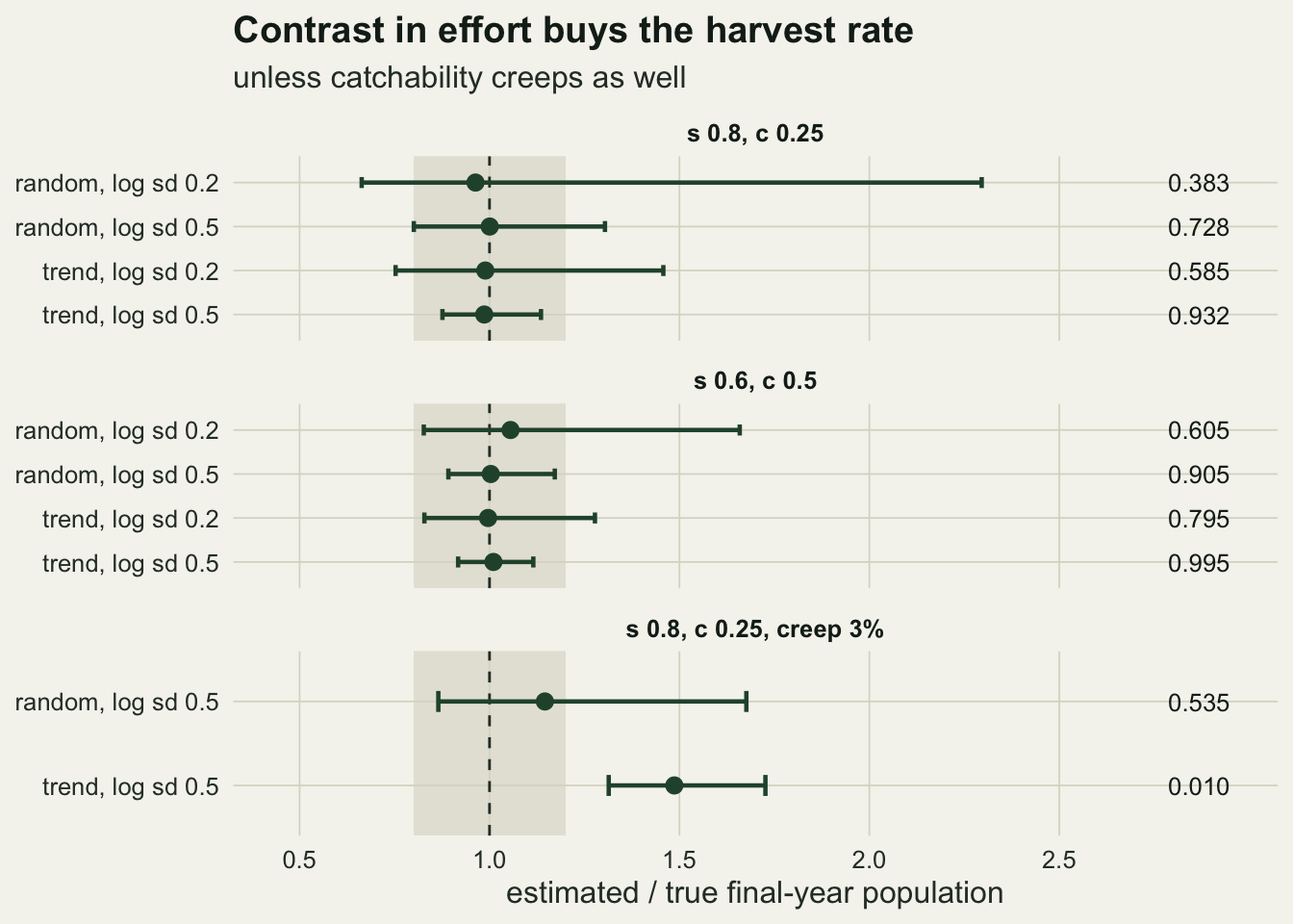
What to report
State where the harvest rate came from before anything else. In a cohort analysis it is an input, and the final-year population is the final harvest divided by it, so the number reported for the present year is the assumption restated. Showing the reconstruction under two or three terminal rates is honest; a single line is not.
For a statistical reconstruction without effort data, report the profile of the harvest rate, not a point estimate: at constant effort it is flat up to the value where survival would reach one. Never report optimiser output at constant effort, from one start or the best of several. If a prior on the harvest rate carries the estimate, say so and show prior and posterior on the same axis; where they coincide, the reconstructed abundance is a transformation of the prior.
With effort data, report the contrast the effort series actually has, as a log standard deviation or a fold range, and the profile of c. Here a log standard deviation of 0.5 put most tables within 20 per cent under both constructions, while at 0.2 with random effort 0.617 of them fell outside; those shares belong to this simulated herd. Then say what is known about catchability through the series. A change in weapons, baiting rules, season timing or access that raises the harvest per hunter-day looks, to this model, like the effort series itself.
Honest limits
The simulated population is the simplest one that carries the problem. Harvest probability is the same at every age, survival is the same at every age and year, recruitment varies but has no density dependence, and animals leave the table after the sixth class instead of accumulating in a plus group. Real reconstructions separate the sexes and let vulnerability differ by age. That does not remove the ridge: if every age has its own vulnerability and survival, multiplying all harvest probabilities by one factor and adjusting each survival and each cohort size to match keeps every expected count at constant effort, as long as no survival passes one. The shares in the replicate study, though, are for this herd and would move with every one of these choices.
Effort is known exactly here, and so is natural survival in the cohort analysis. Hunter-days from licence returns are themselves estimates, and error in the effort series shrinks the contrast that identifies c towards the constant-effort case; how fast was not measured. Natural survival is assumed in practice too, as natural mortality is in fisheries, and an error in it adds a second bias to every back-calculated year, which the terminal guess can neither reveal nor correct; its size was not measured either.
The Bayesian section multiplies a prior on the harvest rate by a profile likelihood. That is not the hierarchical model of Bellier and colleagues, whose superpopulation formulation, priors and age structure all differ, and nothing above tests their results. What carries over is that at constant effort the conditional part of any likelihood built on the age-at-harvest table alone is flat along the ridge, so the harvest rate it returns comes from elsewhere: from the prior, or from the treatment of the cohort sizes, which can tilt it in either direction, or not at all, depending on that choice.
The replicate study used the best of three starts for each fit. At a log standard deviation of 0.2 the bowl is shallow, and in 0.055 of the random-effort fits at the main point the three starts ended more than 0.01 log-likelihood units apart (0.015 at most in the other designs). Where starts disagree, the best of three is still only the best of three, and a wider search could move some of those tables. The catchability creep was run at one rate, 3 per cent a year, with one declining and one random effort series.
References
Fry FEJ 1949 Biometrics 5(1):27-67 (10.2307/3001890)
Gove NE, Skalski JR, Zager P, Townsend RL 2002 Journal of Wildlife Management 66(2):310-320 (10.2307/3803163)
Bellier E, Ferreira DC, Kalb DM, Ganoe LS, Mayer AE, Gerber BD 2024 Ecosphere 15(6):e4878 (10.1002/ecs2.4878)