library(ggplot2)
library(patchwork)
library(mgcv)

te_paper  <- "#f5f4ee"
te_ink    <- "#16241d"
te_body   <- "#2c3a31"
te_forest <- "#275139"
te_rust   <- "#b5534e"
te_gold   <- "#c9b458"
te_line   <- "#dad9ca"

theme_datasheet <- function() {
  theme_minimal(base_size = 12) +
    theme(plot.background  = element_rect(fill = te_paper, colour = NA),
          panel.background = element_rect(fill = te_paper, colour = NA),
          panel.grid.major = element_line(colour = te_line, linewidth = 0.3),
          panel.grid.minor = element_blank(),
          text             = element_text(colour = te_body),
          plot.title       = element_text(colour = te_ink, face = "bold"),
          plot.subtitle    = element_text(colour = te_body),
          axis.text        = element_text(colour = te_body))
}Tuned shrinkage and the penalty your data needed
R
regularisation
species distribution models
calibration
simulation
ecology tutorial
Cross-validated ridge is right on average and wrong per dataset. Simulating in R why a species model’s tuned penalty ranks opposite to the one its data needed.
A few hundred plots surveyed for a ground-nesting bird, a few dozen presences, and ten standardised habitat covariates that somebody thought might matter. Ten predictors against that many presences is where this site, and most of the literature, sends people to a penalty: fit a ridge logistic regression and let cross-validation decide how hard to shrink. The post on ridge regression tunes its penalty by generalised cross-validation and ten-fold cross-validation on one dataset and is careful to add that “neither is guaranteed to recover the penalty that minimises true error.” This post measures how far from that penalty the tuner lands, survey by survey.
The closest relative here is the post on regularisation in MaxEnt. It asks what regularisation multiplier is right for a given number of records, and to answer it, it sweeps the multiplier, averages the held-out curves over replicate datasets and only then takes the maximum. That gives the penalty that is right on average for that many records. Its closing section goes one step further and shows that a multiplier tuned on a 40-record split scatters widely from dataset to dataset and does not locate that optimum. What it does not ask is whether the scatter tracks each dataset’s own needed penalty: whether the datasets that got a small penalty were the ones that needed one. This post asks that question: whether the penalty your own cross-validation picked is the one your own data needed. Across simulated surveys the two are ranked in opposite orders, at about 40 presences and still at about 150, and what the small sample adds is the price.
It is also not the question in data leakage in model validation, whose section on choosing a model on the folds you report shows that the cross-validated error of a tuned model is “a minimum over many noisy estimates”, biased downwards. That is about the number reported for a tuned model; here the number is honest and the question is whether the chosen penalty was the right one. And it is the opposite design choice to checking a penalised regression, which holds its penalty fixed so that the experiment stays about inference rather than tuning. The yardstick throughout is the calibration slope of Cox 1958, which is the slope of the same logistic regression of outcome on the logit of the prediction that the calibration post fits for Platt scaling, fitted here on test sites instead of used as a repair.
None of the result is new. Sinkovec, Heinze, Blagus and Geroldinger 2021 compared tuned and pre-specified ridge penalties for logistic regression in small or sparse data and report that the penalties optimised in small datasets are negatively correlated with the optimal ones. Van Calster, van Smeden, De Cock and Steyerberg 2020 found, across several shrinkage methods, that shrinkage improved the calibration slope on average while the correlation between the estimated and the optimal shrinkage was typically negative. Riley, Snell, Martin and colleagues 2021 showed that tuning parameters are estimated with large uncertainty and that the uncertainty turns into miscalibration in new data, worst when the sample is small. The first two report the dataset-by-dataset anti-correlation itself; the third reports the uncertainty and its cost. This post is a demonstration of those results in a species distribution design, not a claim to them. What it measures is the rank correlation at presence counts that ecologists actually have, cross-validation against restricted maximum likelihood (REML) as the tuner, the spread of the calibration slope against the spread an oracle achieves, and the fact that the reversal is still there at four times the data, where it costs almost nothing.
One species, ten covariates, a hundred surveys
Each simulated survey is one set of plots. The ten covariates are standard normal with a pairwise correlation of 0.3, as habitat variables measured on the same plots usually are. Three of them carry real effects on the logit scale, 0.9, -0.6 and 0.4 per standard deviation, and the other seven carry nothing. The intercept is -2.6, and each survey is sized by dividing its presence target by 0.11 and rounding, so a survey aimed at 40 presences has 364 plots and one aimed at 160 has four times as many. A survey with fewer than 8 presences is redrawn. The same population also supplies one test set of 10000 plots per presence level, which is where every calibration slope and every test deviance is computed.
p_pred    <- 10                                  # standardised habitat covariates
beta_true <- c(0.9, -0.6, 0.4, rep(0, p_pred - 3))
b0_true   <- -2.6                                # intercept; the prevalence is checked below
rho       <- 0.3                                 # pairwise correlation of the covariates
prev_set  <- 0.11
min_pres  <- 8                                   # datasets with fewer presences are redrawn
n_test    <- 10000                               # test sites per presence level
n_ds      <- 100                                 # datasets per main presence level
n_pilot   <- 50                                  # pilot surveys per level, fixed-penalty bound
target_extra <- c(20, 80); n_extra <- 50         # two further presence levels
lam_grid  <- c(0, 10^seq(-2, 2.5, length.out = 19))
lam_floor <- 10^-2.5                             # where lambda = 0 sits for ranking
lam_ip    <- 2                                   # Sinkovec et al.: odds ratio 1/4 to 4
lam_wp    <- 0.5                                 # Sinkovec et al.: odds ratio 1/16 to 16

draw_sites <- function(n) {
  X <- matrix(rnorm(n * p_pred), n) * sqrt(1 - rho) + rnorm(n) * sqrt(rho)
  list(X = X, y = rbinom(n, 1, plogis(b0_true + drop(X %*% beta_true))))
}
draw_survey <- function(n) {
  repeat { d <- draw_sites(n); if (sum(d$y) >= min_pres) return(d) }
}
set.seed(1301)
prev_check <- mean(draw_sites(200000)$y)
p_redraw <- pbinom(min_pres - 1, round(20 / prev_set), prev_check)
On 200000 simulated plots the prevalence is 0.099, a little below the 0.11 used to size the surveys, so they come in slightly under their presence targets; the medians are given with every result. The redraw rule conditions every result on at least 8 presences; it is part of the design, but it hardly ever binds: even at the smallest level used below, aimed at 20 presences, the binomial chance of falling below 8 is 0.20 per cent.
The fits are written out in base R, in the style of the sibling post on centring a quadratic before the penalty. The covariates are standardised inside each fit and the penalty acts on the standardised slopes, with the intercept left free. Ridge logistic regression is penalised iteratively reweighted least squares: it minimises minus the log-likelihood plus half the penalty times the sum of squared slopes, on a grid of 20 penalties, zero and 19 values evenly spaced in log from 0.01 to 10^2.5, each fit starting from the next larger penalty’s solution.
Four ways of choosing the penalty get the same survey. Five-fold cross-validation picks the grid penalty with the smallest summed held-out deviance, standardising inside each training fold. REML treats the ten slopes as draws from one normal distribution with a shared variance and estimates that variance, which mgcv does through paraPen with its Laplace approximation for a binomial response. The heuristic factor of van Houwelingen and le Cessie 1990 is not a ridge penalty at all: it multiplies the unpenalised slopes by (chi2 - df) / chi2, where chi2 is the likelihood ratio statistic of the unpenalised fit against the null model and df is the number of slopes, and then re-estimates the intercept. The fourth is a penalty fixed in advance, and its rule is taken from Sinkovec and colleagues 2021 as published: a ridge penalty is a normal prior on each standardised coefficient with variance one over the penalty, and a 95 per cent prior interval of 1/4 to 4 for the odds ratio per standard deviation gives a prior variance of 1/2 and a penalty of 2 (their informative prior); an interval of 1/16 to 16 gives a penalty of 1/2 (their weakly informative prior).
The target is an oracle. For each survey the whole grid is fitted, every fit is scored on the 10000 test plots, and the penalty with the smallest test deviance is the one that survey needed. Sinkovec and colleagues choose the penalty of their prediction oracle against the true event probabilities instead; test deviance is the version an ecologist scoring predictions would recognise, and a second oracle, the grid penalty whose calibration slope is nearest 1, is reported beside it further down.
standardise_cols <- function(X) {
  ctr <- colMeans(X); Xc <- sweep(X, 2, ctr)
  scl <- sqrt(colMeans(Xc^2))                 # n divisor, as in the sibling posts
  list(Z = sweep(Xc, 2, scl, "/"), ctr = ctr, scl = scl)
}
to_raw_scale <- function(b_std, st) {         # intercept + standardised slopes -> raw scale
  c(b_std[1] - sum(b_std[-1] / st$scl * st$ctr), b_std[-1] / st$scl)
}
# penalised IRLS: minimise -loglik + (lambda / 2) ||b||^2, intercept unpenalised
ridge_logit <- function(Z, y, lambda, b = NULL) {
  Z1 <- cbind(1, Z); P <- diag(c(0, rep(lambda, ncol(Z))))
  if (is.null(b)) b <- c(qlogis(mean(y)), rep(0, ncol(Z)))
  for (it in 1:100) {
    eta <- drop(Z1 %*% b); mu <- plogis(eta); w <- pmax(mu * (1 - mu), 1e-10)
    b_new <- drop(solve(crossprod(Z1, Z1 * w) + P, crossprod(Z1, w * eta + (y - mu))))
    if (max(abs(b_new - b)) < 1e-9) return(b_new)
    b <- b_new
  }
  b
}
ridge_path <- function(X, y, lambdas = lam_grid) {   # raw-scale coefficients, one column per lambda
  st <- standardise_cols(X); B <- matrix(0, ncol(X) + 1, length(lambdas)); b <- NULL
  for (j in rev(seq_along(lambdas))) {
    b <- ridge_logit(st$Z, y, lambdas[j], b); B[, j] <- to_raw_scale(b, st)
  }
  B
}
deviance_of <- function(B, X, y) {
  mu <- plogis(cbind(1, X) %*% B); mu <- pmin(pmax(mu, 1e-12), 1 - 1e-12)
  unname(-2 * colSums(y * log(mu) + (1 - y) * log(1 - mu)))
}
fit_ridge_cv <- function(X, y, folds, lambdas = lam_grid) {   # 5-fold CV deviance
  cv_dev <- numeric(length(lambdas))
  for (k in seq_len(max(folds))) {
    tr <- folds != k
    cv_dev <- cv_dev + deviance_of(ridge_path(X[tr, ], y[tr], lambdas), X[!tr, , drop = FALSE], y[!tr])
  }
  k <- which.min(cv_dev); list(lambda = lambdas[k], k = k)
}
# ridge with one shared prior variance for the ten slopes, tuned by REML in mgcv
fit_ridge_reml <- function(X, y) {
  st <- standardise_cols(X); Z <- st$Z
  g <- gam(y ~ Z, family = binomial, paraPen = list(Z = list(diag(ncol(Z)))), method = "REML")
  list(coef = to_raw_scale(unname(coef(g)), st), lambda = unname(g$sp[1]))
}
# uniform shrinkage of the MLE slopes by (chi2 - df) / chi2, intercept re-estimated
fit_heuristic <- function(X, y, b_mle) {
  b_null <- c(qlogis(mean(y)), rep(0, ncol(X)))
  chi2 <- deviance_of(cbind(b_null), X, y) - deviance_of(cbind(b_mle), X, y)
  s_fac <- max(0, (chi2 - ncol(X)) / chi2)
  lp <- drop(X %*% b_mle[-1]) * s_fac
  a0 <- coef(glm(y ~ offset(lp), family = binomial))[1]
  list(coef = c(unname(a0), s_fac * b_mle[-1]), shrink = s_fac, chi2 = chi2)
}
# calibration slope on the test sites: logistic regression of y on the linear predictor
cal_slopes <- function(B, X, y) {
  eta <- cbind(1, X) %*% B
  apply(eta, 2, function(e) {
    if (sd(e) < 1e-10) return(NA_real_)
    ab <- c(0, 1)
    for (it in 1:50) {
      m <- plogis(ab[1] + ab[2] * e); w <- m * (1 - m)
      H <- matrix(c(sum(w), sum(w * e), sum(w * e), sum(w * e^2)), 2)
      stp <- tryCatch(solve(H, c(sum(y - m), sum((y - m) * e))), error = function(err) c(NA, NA))
      if (anyNA(stp)) return(NA_real_)
      ab <- ab + stp; if (max(abs(stp)) < 1e-10) return(ab[2])
    }
    NA_real_
  })
}
log_lam <- function(l) log10(pmax(l, lam_floor))
Three pieces are checked against an outside reference before anything is measured. At a penalty of zero the IRLS fit should reproduce glm. The REML penalty from mgcv is only comparable with the grid if the two parameterise the penalty the same way, so refitting the IRLS at the penalty mgcv reports should return the coefficients mgcv reports. And the hand-coded calibration slope should match the slope glm gives for the same regression.
set.seed(2210)
chk <- draw_survey(364)
b_glm <- unname(coef(glm(chk$y ~ chk$X, family = binomial)))
gap_mle <- max(abs(ridge_path(chk$X, chk$y, 0)[, 1] - b_glm))
rm_chk <- fit_ridge_reml(chk$X, chk$y)
b_at_reml <- ridge_path(chk$X, chk$y, rm_chk$lambda)[, 1]
gap_reml <- max(abs(b_at_reml - rm_chk$coef))
cal_chk <- cal_slopes(cbind(b_glm), chk$X, chk$y)
gap_cal <- abs(cal_chk - unname(coef(glm(chk$y ~ drop(cbind(1, chk$X) %*% b_glm), family = binomial))[2]))
The unpenalised fit matches glm to \(8.2 \times 10^{-10}\), the IRLS refit at the REML penalty of 27.1 matches the mgcv coefficients to \(3.1 \times 10^{-15}\), and the calibration slope matches glm to \(6.7 \times 10^{-10}\). The REML penalties below are therefore on the same scale as the grid.
one_survey <- function(n, test, lam_fixed_opt) {
  d <- draw_survey(n); X <- d$X; y <- d$y
  folds <- sample(rep(1:5, length.out = n))
  B <- ridge_path(X, y)
  td <- deviance_of(B, test$X, test$y) / length(test$y)
  cs_grid <- cal_slopes(B, test$X, test$y)
  cv <- fit_ridge_cv(X, y, folds)
  rm <- suppressWarnings(fit_ridge_reml(X, y))
  hu <- suppressWarnings(fit_heuristic(X, y, B[, 1]))
  st <- standardise_cols(X)
  fixed <- sapply(c(lam_ip, lam_wp, lam_fixed_opt), function(l) to_raw_scale(ridge_logit(st$Z, y, l), st))
  extra <- cbind(rm$coef, hu$coef, fixed)
  td_x <- deviance_of(extra, test$X, test$y) / length(test$y)
  cs_x <- cal_slopes(extra, test$X, test$y)
  j_or <- which.min(td); j_cs <- which.min(abs(cs_grid - 1))
  c(pres = sum(y), chi2 = hu$chi2, l_cv = lam_grid[cv$k], l_or = lam_grid[j_or], l_cs = lam_grid[j_cs],
    l_reml = rm$lambda, s_heur = hu$shrink,
    cs_mle = cs_grid[1], cs_cv = cs_grid[cv$k], cs_or = cs_grid[j_or], cs_reml = cs_x[1], cs_heur = cs_x[2],
    cs_ip = cs_x[3], cs_wp = cs_x[4], cs_opt = cs_x[5],
    ex_mle = td[1] - td[j_or], ex_cv = td[cv$k] - td[j_or], ex_reml = td_x[1] - td[j_or],
    ex_heur = td_x[2] - td[j_or], ex_ip = td_x[3] - td[j_or], ex_wp = td_x[4] - td[j_or],
    ex_opt = td_x[5] - td[j_or])
}
One more arm needs a number fixed before the main run. A fixed penalty set at the right value is the best a fixed penalty could possibly do, and it is worth having as a bound. The right value is taken from an independent pilot population, a different seed from everything below: 50 surveys per presence level, each with its own test-deviance oracle, and the median of those oracles. A real analyst never has this number. It enters the tables as an optimistic bound and is labelled that way everywhere.
target_main <- c(40, 160)
n_sites <- function(target) round(target / prev_set)
set.seed(5150)
lam_opt <- sapply(target_main, function(tg) {
  test_p <- draw_sites(n_test)
  median(replicate(n_pilot, {
    d <- draw_survey(n_sites(tg))
    lam_grid[which.min(deviance_of(ridge_path(d$X, d$y), test_p$X, test_p$y))]
  }))
})
The pilot median is a penalty of 10.00 at the smaller presence level and 3.16 at the larger. The main run then draws 100 surveys at each level, with one test set per level, and fits all eight arms to every survey: no penalty, cross-validated ridge, REML ridge, the heuristic factor, the two Sinkovec penalties, the pilot-optimum penalty and the oracle.
Right on average
t_start <- proc.time()
set.seed(4027)
runs <- lapply(seq_along(target_main), function(i) {
  test <- draw_sites(n_test)
  as.data.frame(t(replicate(n_ds, one_survey(n_sites(target_main[i]), test, lam_opt[i]))))
})
names(runs) <- c("small", "large")
t_main <- (proc.time() - t_start)[["user.self"]]

sp_boot <- function(a, b, n_boot = 2000) {
  est <- cor(a, b, method = "spearman")
  bs <- replicate(n_boot, { i <- sample.int(length(a), replace = TRUE); cor(a[i], b[i], method = "spearman") })
  c(est = est, lo = unname(quantile(bs, 0.025)), hi = unname(quantile(bs, 0.975)))
}
set.seed(77)
sp_tab <- lapply(runs, function(R) rbind(
  cv_or   = sp_boot(log_lam(R$l_cv), log_lam(R$l_or)),
  reml_or = sp_boot(log_lam(R$l_reml), log_lam(R$l_or)),
  cv_cs   = sp_boot(log_lam(R$l_cv), log_lam(R$l_cs)),
  reml_cs = sp_boot(log_lam(R$l_reml), log_lam(R$l_cs)),
  heur    = sp_boot(R$s_heur, R$cs_mle)))
q10 <- function(v) unname(quantile(v, 0.1, na.rm = TRUE))
q90 <- function(v) unname(quantile(v, 0.9, na.rm = TRUE))
arms <- c("mle", "cv", "reml", "heur", "ip", "wp", "opt", "or")
cs_summary <- lapply(runs, function(R) t(sapply(arms, function(a) {
  v <- R[[paste0("cs_", a)]]
  c(med = median(v, na.rm = TRUE), lo = q10(v), hi = q90(v),
    over = mean(v > 1.25, na.rm = TRUE), under = mean(v < 0.8, na.rm = TRUE), n_na = sum(is.na(v)))
})))
ex_summary <- lapply(runs, function(R) sapply(setdiff(arms, "or"), function(a) median(R[[paste0("ex_", a)]])))
pres_med <- sapply(runs, function(R) median(R$pres))
mcse_max <- sqrt(0.25 / n_ds)
cs_at <- function(lev, a, what) cs_summary[[lev]][a, what]
sp_at <- function(lev, what, k = "est") sp_tab[[lev]][what, k]
ex_at <- function(lev, a) ex_summary[[lev]][[a]]
tie_or0 <- sapply(runs, function(R) mean(R$l_or == 0))
tie_cv0 <- sapply(runs, function(R) mean(R$l_cv == 0))
tie_cvtop <- sapply(runs, function(R) mean(R$l_cv == max(lam_grid)))
tie_ortop <- sapply(runs, function(R) mean(R$l_or == max(lam_grid)))
sp_nz <- sapply(runs, function(R) { k <- R$l_or > 0
  c(n = sum(k), cv = cor(log_lam(R$l_cv[k]), log_lam(R$l_or[k]), method = "spearman"),
    reml = cor(log_lam(R$l_reml[k]), log_lam(R$l_or[k]), method = "spearman")) })
reml_rng <- sapply(runs, function(R) range(R$l_reml))
lam_med <- sapply(runs, function(R) c(cv = median(R$l_cv), reml = median(R$l_reml), or = median(R$l_or)))
The surveys have a median of 37 presences on 364 plots at the smaller level and 145 on 1455 at the larger. Start with what tuning is supposed to do. At the smaller level the unpenalised fit has a median calibration slope of 0.693: its predictions are too extreme, the familiar signature of overfitting, and 82 per cent of surveys fall below 0.8. Cross-validated ridge moves the median to 0.969 and REML ridge to 0.994. The median excess test deviance over the oracle, per test plot, falls from 0.0115 without a penalty to 0.0021 with the cross-validated one and 0.0018 with REML, so the tuned penalty removes 82 per cent of the unpenalised fit’s median excess. Even the typical penalty is right: the median cross-validated choice is 10.00, the median REML choice 8.03 and the median oracle 10.00. On average, which is the view of the MaxEnt post’s sample-size sweep, tuning does its job.
Wrong survey by survey
lev_lab <- c(small = "about 40 presences", large = "about 150 presences")
scat <- do.call(rbind, lapply(names(runs), function(lev) {
  R <- runs[[lev]]
  rbind(data.frame(level = lev_lab[[lev]], tuner = "5-fold CV", oracle = log_lam(R$l_or), tuned = log_lam(R$l_cv)),
        data.frame(level = lev_lab[[lev]], tuner = "REML", oracle = log_lam(R$l_or), tuned = log_lam(R$l_reml)))
}))
scat$level <- factor(scat$level, levels = lev_lab)
lab_sp <- do.call(rbind, lapply(names(runs), function(lev) data.frame(
  level = factor(lev_lab[[lev]], levels = lev_lab), tuner = c("5-fold CV", "REML"),
  txt = sprintf("Spearman %.2f", c(sp_at(lev, "cv_or"), sp_at(lev, "reml_or"))))))
set.seed(11)
p_scat <- ggplot(scat, aes(oracle, tuned)) +
  geom_abline(slope = 1, intercept = 0, colour = te_body, linetype = "dashed", linewidth = 0.5) +
  geom_jitter(aes(colour = tuner), width = 0.06, height = 0, alpha = 0.7, size = 1.8) +
  geom_text(data = lab_sp, aes(x = -2.4, y = 2.45, label = txt), hjust = 0, vjust = 1, size = 3.6,
            colour = te_ink) +
  facet_grid(tuner ~ level) +
  scale_colour_manual(values = c("5-fold CV" = te_forest, "REML" = te_rust), guide = "none") +
  coord_cartesian(xlim = c(-2.5, 2.5), ylim = c(-2.5, 2.5)) +
  labs(x = "log10 penalty the dataset needed (test-deviance oracle; 0 plotted at -2.5)",
       y = "log10 penalty the tuner chose",
       title = "The tuned penalty against the needed one",
       subtitle = "one point per simulated survey, 100 per panel; dashed line: tuned = needed") +
  theme_datasheet() +
  theme(strip.text = element_text(colour = te_ink, face = "bold"))
p_scat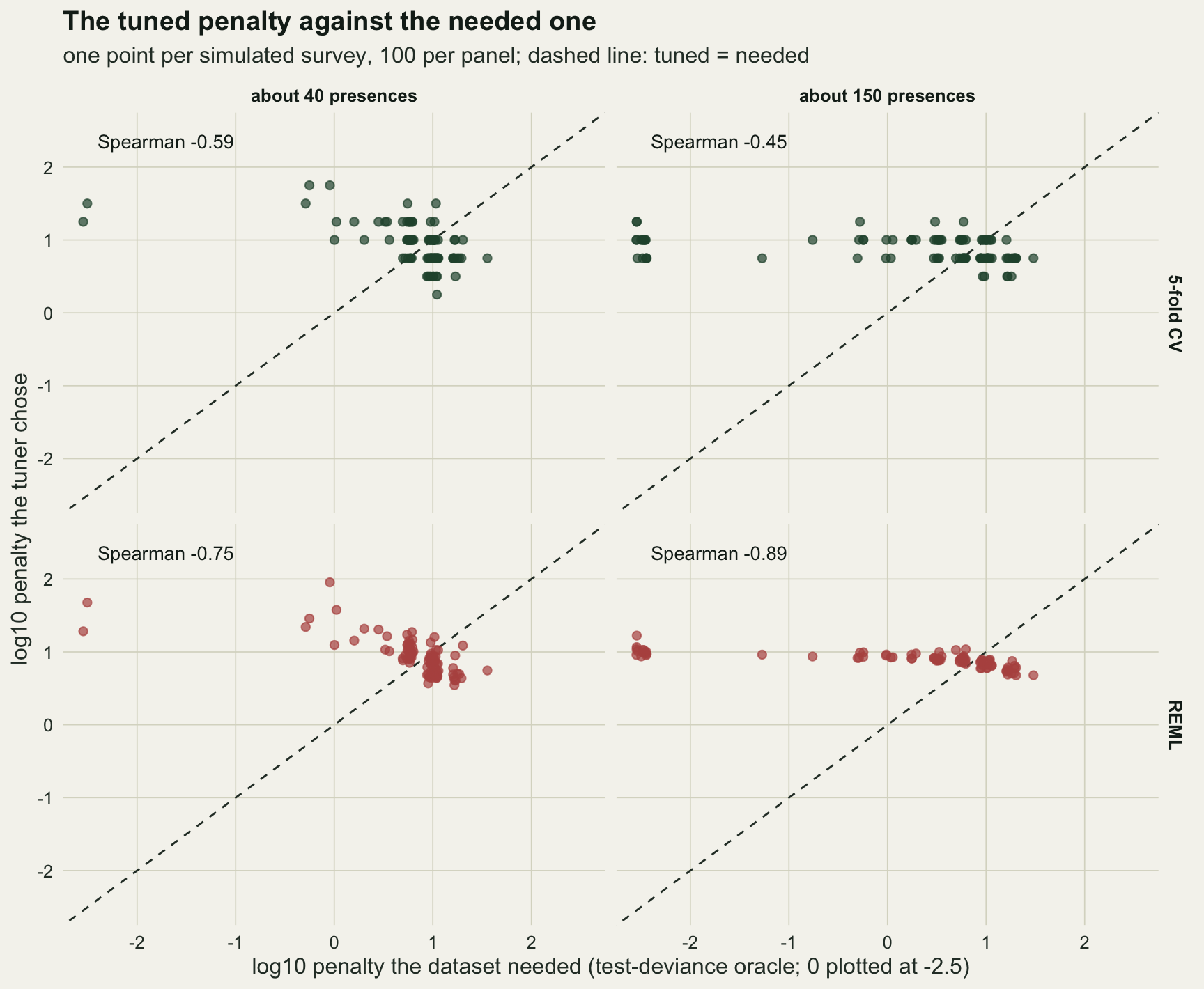
Survey by survey it does not. At 37 presences the Spearman correlation between the log penalty cross-validation chose and the log penalty the survey needed is -0.59, with a 95 per cent bootstrap interval over surveys of -0.70 to -0.46. Broadly, the surveys that needed more shrinkage got less. REML does not rescue it: its correlation is -0.75 (-0.84 to -0.64), stronger in the wrong direction. For the ranking, a penalty of zero is placed at 10^-2.5, below the grid; the oracle chose zero in 2 per cent of surveys at this level, and cross-validation picked the bottom end of the grid in 0 per cent and the top end in 0 per cent, so the ties at the grid ends do not drive the number.
The cost shows in the calibration slope. The oracle keeps it between 0.91 and 1.11 from the 10th to the 90th percentile. Cross-validated ridge spreads it from 0.75 to 1.48, and 23 per cent of surveys end over-shrunk (slope above 1.25, predictions too timid) while 22 per cent end under-shrunk (slope below 0.8, predictions still too extreme); for the oracle those shares are 0 and 1 per cent. REML spreads it from 0.74 to 1.41. With 100 surveys the Monte Carlo standard error of any of these shares is at most 0.05. A median of 0.969 made of slopes that far apart is the “right on average, wrong in the dataset you have” pattern of Van Calster and colleagues, in an ecological design.
The REML penalties are worth a sentence, because the sibling post on centring found REML ridge collapsing to the boundary where the shared variance is zero and every slope is shrunk away. That happened there because the coding made two coefficients far larger than the rest. No coding does that here, and nothing of the sort happens at the two main levels: the REML penalty ranges from 3.5 to 90.2 at the smaller level and from 4.8 to 16.7 at the larger, and no fit there reaches the boundary. Its failure here is the same one cross-validation has, not a collapse.
Why the ranking reverses
Both tuners read the data’s apparent signal. A survey whose noise happens to line up with the covariates looks strong: its unpenalised coefficients are large and its likelihood ratio statistic is high. Cross-validation sees held-out plots that the covariates predict well and asks for little shrinkage; REML sees large coefficients and estimates a large shared variance, which is a small penalty. But that same survey is the one whose coefficients are most inflated by the noise, so it is the one that needed the most shrinkage. The likelihood ratio statistic of the unpenalised fit is a direct measure of apparent signal and puts the whole mechanism on one axis.
R_s <- runs$small
sp_chi_cv <- cor(R_s$chi2, log_lam(R_s$l_cv), method = "spearman")
sp_chi_reml <- cor(R_s$chi2, log_lam(R_s$l_reml), method = "spearman")
sp_chi_or <- cor(R_s$chi2, log_lam(R_s$l_or), method = "spearman")
sp_chi_csmle <- cor(R_s$chi2, R_s$cs_mle, method = "spearman")
chi_split <- median(R_s$chi2)
lo_half <- R_s$chi2 <= chi_split
med_by_half <- rbind(cv = tapply(R_s$l_cv, lo_half, median), or = tapply(R_s$l_or, lo_half, median),
                     csmle = tapply(R_s$cs_mle, lo_half, median))
mech <- rbind(data.frame(chi2 = R_s$chi2, lam = log_lam(R_s$l_cv), who = "chosen by 5-fold CV"),
              data.frame(chi2 = R_s$chi2, lam = log_lam(R_s$l_or), who = "needed (oracle)"))
p_mech_a <- ggplot(mech, aes(chi2, lam, colour = who)) +
  geom_point(alpha = 0.7, size = 1.8) +
  geom_smooth(method = "loess", formula = y ~ x, se = FALSE, linewidth = 0.9, span = 0.9) +
  scale_colour_manual(values = c("chosen by 5-fold CV" = te_forest, "needed (oracle)" = te_gold), name = NULL) +
  scale_x_log10() +
  labs(x = "apparent signal (LR chi-squared, no penalty)",
       y = "log10 penalty", title = "Same axis, opposite slopes",
       subtitle = "about 40 presences, 100 surveys") +
  theme_datasheet() + theme(legend.position = "bottom")
p_mech_b <- ggplot(data.frame(chi2 = R_s$chi2, cs = R_s$cs_mle), aes(chi2, cs)) +
  geom_hline(yintercept = 1, colour = te_body, linetype = "dashed", linewidth = 0.5) +
  geom_point(colour = te_rust, alpha = 0.7, size = 1.8) +
  scale_x_log10() +
  labs(x = "apparent signal (same axis)", y = "calibration slope of the unpenalised fit",
       title = "Strong-looking surveys overfit most", subtitle = "slope below 1: predictions too extreme") +
  theme_datasheet()
p_mech_a + p_mech_b + plot_layout(widths = c(1, 1)) + plot_annotation(theme = theme_datasheet())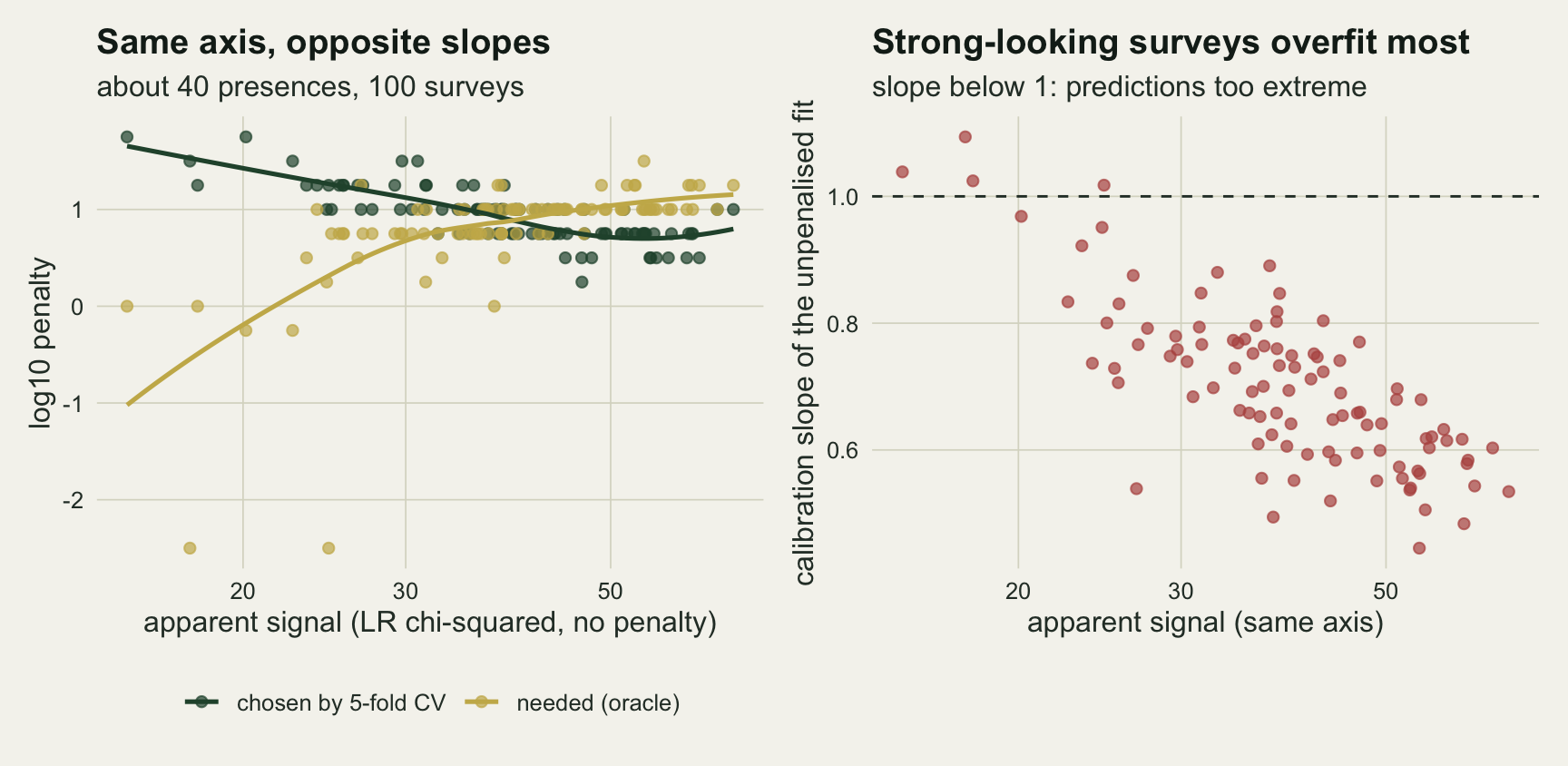
At 37 presences the Spearman correlation of the apparent signal with the cross-validated log penalty is -0.76, with the REML log penalty -0.93, and with the needed log penalty 0.70. Split the surveys at the median apparent signal: in the stronger-looking half the median cross-validated penalty is 5.62 and the median needed penalty 10.00; in the weaker-looking half the two medians swap, 10.00 chosen against 5.62 needed. The right panel shows why the needed penalty rises with apparent signal. The calibration slope of the unpenalised fit falls as the apparent signal grows (Spearman -0.72), with a median of 0.62 in the stronger-looking half and 0.77 in the weaker.
The heuristic factor makes the mechanism explicit, because it is a formula in the apparent signal and nothing else: (chi2 - df) / chi2 grows with chi2, so it shrinks the strongest-looking surveys least by construction. The shrinkage a survey needed from a uniform factor is its unpenalised calibration slope, and the Spearman correlation of the heuristic factor with that slope is -0.72. It equals the correlation of the apparent signal with the same slope, as it must for a monotone function of chi2. The heuristic is a common recommendation for an overfitted small-sample model; it inherits the reversal instead. Van Calster and colleagues included this likelihood-based uniform shrinkage among their methods; here the reason it fails shows on a single axis.
Four times the presences
It is tempting to read the reversal as a small-sample effect that more data will cure. The main run’s larger level, with four times the presences, tests that. Two further levels, aimed at 20 and 80 presences with 50 surveys each and their own test sets, fill in the curve; they carry the same arms, but only the two tuners and the oracle are read from them.
set.seed(6061)
runs_extra <- lapply(seq_along(target_extra), function(i) {
  test <- draw_sites(n_test)
  as.data.frame(t(replicate(n_extra, one_survey(n_sites(target_extra[i]), test, lam_opt[1]))))
})
all_runs <- c(list(runs_extra[[1]], runs$small, runs_extra[[2]], runs$large))
set.seed(78)
sweep_tab <- do.call(rbind, lapply(all_runs, function(R) {
  s_cv <- sp_boot(log_lam(R$l_cv), log_lam(R$l_or)); s_re <- sp_boot(log_lam(R$l_reml), log_lam(R$l_or))
  data.frame(pres = median(R$pres), n = nrow(R),
             tuner = c("5-fold CV", "REML"), sp = c(s_cv[1], s_re[1]), lo = c(s_cv[2], s_re[2]), hi = c(s_cv[3], s_re[3]),
             cs_lo = c(q10(R$cs_cv), q10(R$cs_reml)), cs_hi = c(q90(R$cs_cv), q90(R$cs_reml)),
             or_lo = q10(R$cs_or), or_hi = q90(R$cs_or),
             ex = c(median(R$ex_cv), median(R$ex_reml)), ex_mle = median(R$ex_mle))
}))
sw_at <- function(k, tuner, col) sweep_tab[sweep_tab$tuner == tuner, col][k]
n_excl0 <- sum(sweep_tab$hi < 0)
n_bnd1 <- sum(runs_extra[[1]]$l_reml > 1e4)            # REML fits at the boundary, smallest level
n_na1 <- sum(is.na(runs_extra[[1]]$cs_reml))
lam_bnd1 <- max(runs_extra[[1]]$l_reml)
t_all <- (proc.time() - t_start)[["user.self"]]
At 145 presences the cross-validated correlation is -0.45 (-0.60 to -0.28) and the REML correlation -0.89 (-0.93 to -0.83). The ranking is still reversed with four times the data, and for REML more firmly than before. The oracle chose zero in 15 per cent of surveys at this level, so here the ties at the bottom of the grid are a real share of the ranking; dropping those surveys leaves 85 surveys, with correlations of -0.47 for cross-validation and -0.86 for REML (at the smaller level, -0.57 and -0.73 on 98 surveys). What the extra presences buy is a narrower miss: the cross-validated calibration slope now runs from 0.91 to 1.18 against the oracle’s 0.99 to 1.07, with 2 per cent of surveys over-shrunk and 1 per cent under-shrunk.
p_sw_a <- ggplot(sweep_tab, aes(pres, sp, colour = tuner)) +
  geom_hline(yintercept = 0, colour = te_body, linetype = "dashed", linewidth = 0.5) +
  geom_errorbar(aes(ymin = lo, ymax = hi), width = 0.04, linewidth = 0.5,
                position = position_dodge(width = 0.06)) +
  geom_line(linewidth = 0.9, position = position_dodge(width = 0.06)) +
  geom_point(size = 2.2, position = position_dodge(width = 0.06)) +
  scale_x_log10(breaks = round(sweep_tab$pres[sweep_tab$tuner == "REML"])) +
  scale_colour_manual(values = c("5-fold CV" = te_forest, "REML" = te_rust), name = NULL) +
  labs(x = "median presences per survey", y = "Spearman, tuned against needed",
       title = "The ranking stays reversed", subtitle = "bars: 95 per cent bootstrap intervals over surveys") +
  theme_datasheet() + theme(legend.position = "bottom")
band <- rbind(data.frame(pres = sweep_tab$pres, lo = sweep_tab$cs_lo, hi = sweep_tab$cs_hi, who = sweep_tab$tuner),
              data.frame(pres = unique(sweep_tab$pres), lo = sweep_tab$or_lo[sweep_tab$tuner == "REML"],
                         hi = sweep_tab$or_hi[sweep_tab$tuner == "REML"], who = "oracle"))
p_sw_b <- ggplot(band, aes(pres, colour = who)) +
  geom_hline(yintercept = c(0.8, 1.25), colour = te_body, linetype = "dotted", linewidth = 0.5) +
  geom_errorbar(aes(ymin = lo, ymax = hi), width = 0.06, linewidth = 0.9,
                position = position_dodge(width = 0.09)) +
  scale_x_log10(breaks = round(sweep_tab$pres[sweep_tab$tuner == "REML"])) +
  scale_colour_manual(values = c("5-fold CV" = te_forest, "REML" = te_rust, oracle = te_gold), name = NULL) +
  labs(x = "median presences per survey", y = "calibration slope, 10th to 90th percentile",
       title = "The miss narrows", subtitle = "dotted: the over- and under-shrunk thresholds") +
  theme_datasheet() + theme(legend.position = "bottom")
p_sw_a + p_sw_b + plot_annotation(theme = theme_datasheet())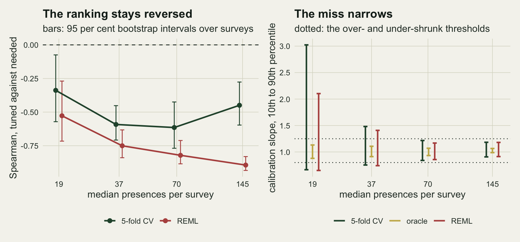
Across the four levels the cross-validated correlation is -0.34, -0.59, -0.61 and -0.45 at median presences of 19, 37, 70 and 145, and the REML correlation -0.53, -0.75, -0.82 and -0.89. Every bootstrap interval excludes zero (8 of 8), and there is no steady drift towards zero as presences accumulate: the cross-validated correlation is weaker at the largest level than at the two middle ones but still clearly negative, and the REML correlation grows stronger at every step. The weakest is cross-validation at the smallest level, where its interval runs from -0.57 to -0.07 on 50 surveys, so even there the reversal holds and the smaller sample makes the ranking noisier rather than stronger.
The price is where the sample size shows. The cross-validated 90th percentile of the calibration slope is 3.02 at the smallest level, 1.48, 1.22 and then 1.18. At the smallest level 1 of the 50 REML fits did reach the boundary (penalty 512161), and its flat prediction has no calibration slope, so the REML percentiles there use the other 49. The median excess test deviance per plot of the cross-validated fit goes from 0.0038 to 0.0004 over the same range, while the unpenalised fit’s goes from 0.0311 to 0.0003. At the largest level both are below 0.001 per plot: the penalty barely matters there, so choosing it the wrong way round barely matters either. That is the whole sample-size story. The reversal does not go away; it stops costing anything.
A fixed penalty, a heuristic factor and a second oracle
If the tuned penalty is anti-correlated with the needed one, a penalty that ignores the data cannot be anti-correlated with anything, and the obvious question is whether it does better. Sinkovec and colleagues recommend exactly that for small or sparse data: fix the degree of shrinkage from prior assumptions about plausible effect sizes. The figure puts all eight arms on the same axis, one point per survey.
arm_lab <- c(mle = "no penalty", cv = "5-fold CV ridge", reml = "REML ridge", heur = "heuristic factor",
             ip = "fixed, Sinkovec IP", wp = "fixed, Sinkovec WP", opt = "fixed at pilot optimum", or = "oracle")
slope_long <- do.call(rbind, lapply(names(runs), function(lev) {
  R <- runs[[lev]]
  do.call(rbind, lapply(arms, function(a) data.frame(level = lev_lab[[lev]], arm = arm_lab[[a]],
                                                   cs = R[[paste0("cs_", a)]])))
}))
slope_long$level <- factor(slope_long$level, levels = lev_lab)
slope_long$arm <- factor(slope_long$arm, levels = rev(arm_lab))
slope_sum <- aggregate(cs ~ level + arm, data = slope_long,
                       FUN = function(v) c(lo = q10(v), med = median(v), hi = q90(v)))
slope_sum <- data.frame(slope_sum[, 1:2], slope_sum$cs)
arm_col <- c("no penalty" = te_body, "5-fold CV ridge" = te_forest, "REML ridge" = te_rust,
             "heuristic factor" = "#8a6d3b", "fixed, Sinkovec IP" = "#5b7f95", "fixed, Sinkovec WP" = "#8fa9b8",
             "fixed at pilot optimum" = "#8a8f7a", "oracle" = te_gold)
p_slopes <- ggplot(slope_long, aes(cs, arm, colour = arm)) +
  annotate("rect", xmin = 0.8, xmax = 1.25, ymin = -Inf, ymax = Inf, fill = te_line, alpha = 0.45) +
  geom_vline(xintercept = 1, colour = te_body, linetype = "dashed", linewidth = 0.5) +
  geom_jitter(width = 0, height = 0.18, alpha = 0.35, size = 1.1) +
  geom_errorbar(data = slope_sum, aes(x = med, xmin = lo, xmax = hi, y = arm), orientation = "y",
                width = 0.5, linewidth = 0.9, inherit.aes = FALSE, colour = te_ink) +
  geom_point(data = slope_sum, aes(x = med, y = arm), inherit.aes = FALSE, colour = te_ink, size = 2.4) +
  facet_wrap(~ level) +
  scale_colour_manual(values = arm_col, guide = "none") +
  scale_x_log10(breaks = c(0.5, 0.8, 1.25, 2, 3)) +
  labs(x = "calibration slope on 10000 test plots (log scale)", y = NULL,
       title = "Calibration slope per survey, eight ways to set the penalty",
       subtitle = "black: median and 10th to 90th percentile; shaded: slope between 0.8 and 1.25") +
  theme_datasheet() +
  theme(strip.text = element_text(colour = te_ink, face = "bold"))
p_slopes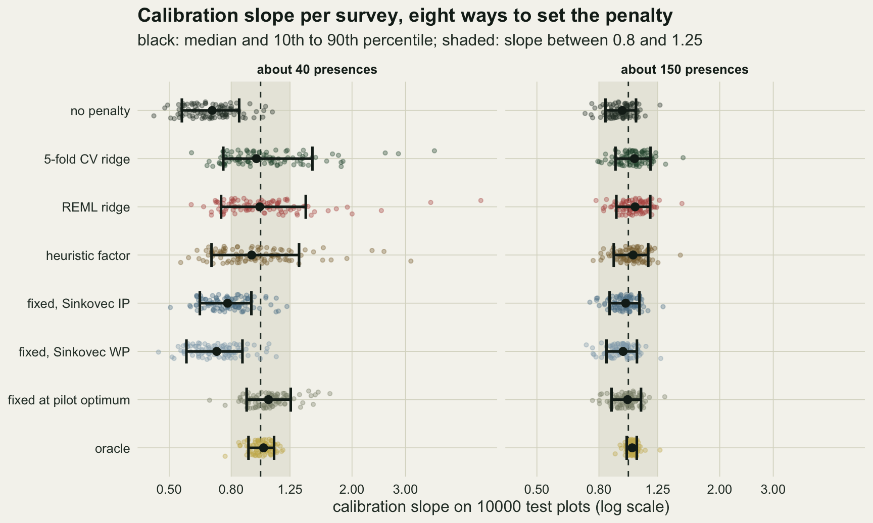
At 37 presences the informative Sinkovec penalty of 2 never over-shrinks (0 per cent of surveys above 1.25), and its calibration slope runs from 0.63 to 0.93, a narrower band than either tuner’s. But the band sits too low: the median slope is 0.779 and 55 per cent of surveys stay under-shrunk. Its median excess test deviance per plot, 0.0055, is about half the unpenalised fit’s 0.0115 and more than twice the cross-validated fit’s 0.0021. The weakly informative penalty of 1/2 shrinks less still, with a median slope of 0.717 and an excess of 0.0094. The reason is the design. The prior interval of 1/4 to 4 is a fair statement about the three real effects, but seven of the ten covariates have no effect at all, and a prior that is honest about the real effects is too generous to the null ones. The penalty these surveys needed was larger.
So the answer to “does a pre-specified penalty beat tuning at 40 presences?” is: in this design, the published rule does not, on the median deviance. It trades the tuners’ two-sided miss for a one-sided under-shrink, which is the safer error if predictions that are too extreme are the thing to avoid. The pilot-optimum penalty of 10.00 shows what a fixed penalty at the right value would do: a median excess of 0.0001 per plot, calibration slopes from 0.90 to 1.26, 11 per cent over-shrunk and 2 per cent under-shrunk, better than every tuned arm. It is an optimistic bound, because the right value came from surveys of the same population scored against its truth, and a real analyst has neither. At 145 presences the informative penalty’s median excess of 0.0002 is below the cross-validated fit’s 0.0004, but at that level every arm’s median excess is below a thousandth of a unit of deviance per plot.
The heuristic factor sits with the tuners, which is what the previous section predicts: its calibration slope runs from 0.69 to 1.34 at the smaller level, with 13 per cent over-shrunk and 30 per cent under-shrunk, and a median excess of 0.0033.
The second oracle changes nothing. Taking the penalty the survey needed as the grid value whose calibration slope is nearest 1, rather than the one with the smallest test deviance, the cross-validated correlation is -0.59 (-0.70 to -0.45) and the REML correlation -0.76 at the smaller level, and -0.40 and -0.86 at the larger. The two definitions of the needed penalty disagree in detail, but both are ranked against the tuners.
What to report
Report how the penalty was chosen and what value it took, and do not read the tuned value as a measurement of how much shrinkage the data needed. In these simulations it is closer to the reverse: a small tuned penalty is a sign that the survey looks strong, and a strong-looking survey at small sample size is the one most likely to be overfitted.
If there is any independent test data, report the calibration slope of the final model on it with its interval, not only a discrimination measure. The slope is the one number that says whether this particular fit shrank too much or too little, and it is the quantity that varies here.
Below something like 50 presences, a penalty fixed in advance from a stated prior, as Sinkovec and colleagues recommend, removes the two-sided miss but is only as good as its prior. Here the published 1/4-to-4 rule never over-shrank, left 55 per cent of surveys under-shrunk and cost 2.6 times the cross-validated fit’s median excess deviance, in a design where seven of the ten covariates had no effect. A prior that reflects how many covariates are expected to matter could do better; the pilot-optimum bound shows how much, with information no analyst has. If you fix the penalty, write down the prior interval for an odds ratio per standard deviation, the penalty it implies and how many covariates you expect to matter, and report the tuned fit beside it.
Do not rely on more data to fix the ranking. At four times the presences the tuned penalty was still ranked against the needed one; what changed was that the whole penalty had stopped mattering. Riley and colleagues reach the same place from the clinical side: they recommend development samples large enough to limit overfitting in the first place, rather than relying on penalisation to remove it.
Honest limits
The design is one logistic model with ten standard normal covariates, three real effects and seven null ones, and one prevalence. The share of null covariates pushes the needed penalty up, which is why the informative Sinkovec penalty under-shrinks here; in a design where every covariate matters, the same rule could land on the right side. The size of every correlation and every share above belongs to this design, and the direction of the reversal is what carries across, because the mechanism only needs a tuner that reads the apparent signal.
MaxEnt-style hinge and product features, and presence-background data with its own loss, were not run. Those are where most species distribution models are fitted, and the MaxEnt post’s own penalty is a per-feature regularisation multiplier, not a ridge. Cross-validation there reads the same apparent signal, so there is no reason to expect the reversal to vanish, but its size with many correlated basis functions per covariate is unmeasured.
The penalties are chosen on a grid of 20 values spaced a quarter of a decade apart, and the oracle is a grid minimum too, so both carry ties and the Spearman correlations are computed with them. The oracle chose a penalty of zero in 2 and 15 per cent of surveys at the two main levels; the second oracle gives the same sign at both. REML is continuous and mgcv’s REML for a binomial response rests on a Laplace approximation, which was not checked against an exact integral.
Each level has one test set, and each survey one draw of the five folds; redrawing the folds would move individual cross-validated penalties, and the effect of that on the correlation was not measured. The main levels are 100 surveys each and the two extra levels 50, with seeds set once when the code was written and not changed after the results were seen. The calibration slope is measured on plots from the same population as the survey. A model moved to a new region has a second source of miscalibration on top of this one, and nothing here measures it.
References
Sinkovec H, Heinze G, Blagus R, Geroldinger A 2021 BMC Medical Research Methodology 21(1):199 (10.1186/s12874-021-01374-y)
Van Calster B, van Smeden M, De Cock B, Steyerberg EW 2020 Statistical Methods in Medical Research 29(11):3166-3178 (10.1177/0962280220921415)
Riley RD, Snell KIE, Martin GP, Whittle R, Archer L, Sperrin M, Collins GS 2021 Journal of Clinical Epidemiology 132:88-96 (10.1016/j.jclinepi.2020.12.005)
van Houwelingen JC, le Cessie S 1990 Statistics in Medicine 9(11):1303-1325 (10.1002/sim.4780091109)
Cox DR 1958 Biometrika 45(3-4):562-565 (10.1093/biomet/45.3-4.562)