library(ggplot2)
library(survival)

te_paper  <- "#f5f4ee"
te_ink    <- "#16241d"
te_body   <- "#2c3a31"
te_forest <- "#275139"
te_rust   <- "#b5534e"
te_gold   <- "#c9b458"
te_line   <- "#dad9ca"

theme_datasheet <- function() {
  theme_minimal(base_size = 12) +
    theme(plot.background  = element_rect(fill = te_paper, colour = NA),
          panel.background = element_rect(fill = te_paper, colour = NA),
          panel.grid.major = element_line(colour = te_line, linewidth = 0.3),
          panel.grid.minor = element_blank(),
          text             = element_text(colour = te_body),
          plot.title       = element_text(colour = te_ink, face = "bold"),
          plot.subtitle    = element_text(colour = te_body),
          axis.text        = element_text(colour = te_body),
          strip.text       = element_text(colour = te_ink))
}Thermal death time and the ramping rate
R
thermal ecology
physiology
survival analysis
censoring
simulation
ecology tutorial
A ramp CTmax moves with the heating rate along the thermal death time line. Designing static knockdown assays in R, and why the survivors must stay in the fit.
Two ground beetles from the same heath are put through the standard heat tolerance assay: a water bath that warms from room temperature at a quarter of a degree per minute until each animal loses its righting response. The temperature at knockdown is the critical thermal maximum, CTmax, and species B comes out more than a degree above species A. The comparison goes into a table of warming tolerances, and species B is filed as the safer of the two. Then a heatwave holds the leaf litter a little above thirty degrees from late morning into the evening, and it is species B that dies.
Nothing in that story needs a measurement error. A heat tolerance limit is a temperature paired with a duration: an animal that shrugs off a minute at one temperature can die within an hour at a temperature several degrees lower. The relation between the two is the thermal death time line, on which the logarithm of survival time falls linearly with temperature, a shape Bigelow (1921) described for bacteria and Rezende and colleagues (2014) set out for animals as a “tolerance landscape” with two parameters: CT1 (their CTmax), the temperature that kills in one minute, and z, the warming that cuts survival time tenfold. A ramp assay is an exposure to a rising temperature, so its CTmax is a point on that landscape chosen by the ramping rate. Terblanche and colleagues (2007) showed in tsetse flies that measured critical limits depend on the ramping rate and the starting temperature, and Jorgensen and colleagues (2021) proposed one model for estimating tolerance limits across static, ramping and fluctuating exposures, in which the ramp CTmax follows from the thermal death time line by summing damage; they also found heat injury additive across two static temperatures in Drosophila melanogaster.
This post is a demonstration of that framework, not a discovery. The ramp formula and the rate at which two species swap rank are closed forms (the ramp formula is Jorgensen and colleagues’ model, written with the one minute parameterisation used here), derived below and checked against a numerical integration of damage; they are reproduced here, not found. The part that is measured is a design question that the formulas raise: to predict tolerance over an eight hour heatwave, z has to be estimated from static assays, and the assays that estimate it well are the long, cool ones in which some animals are still standing when the observer stops watching.
That last point is a censoring problem, and the site already has the tool for it. On this site CTmax has so far been a fixed number: in Thermal performance curves in R it is the upper zero of a fitted performance curve, “an extrapolation to the edge of the curve”, and in Thermal safety margins and warming it is a fixed value per latitude from which the warming tolerance is read off. Neither asks what CTmax depends on in the assay, and that is the question here. The fix for the animals that survive the observation window is the censored likelihood of Values below the detection limit in R, which lets an observation below a limit contribute the probability of being there rather than an invented value. Dropping those animals is the truncation that Germination trials as time-to-event data describes for mean germination time, where a seed enters the mean only if it germinated before the trial stopped. Neither mechanism is new here; the post measures what each costs in a knockdown assay, using survreg as Parametric survival and the AFT model introduces it.
The thermal death time line
Write t(T) for the time, in minutes, that an animal survives at a constant temperature T. The thermal death time line says
log10 t(T) = (CT1 - T) / z,
so at T = CT1 the animal lasts one minute, and every z degrees cooler it lasts ten times longer. Read the other way, the temperature an animal tolerates for a given duration is CT1 - z log10 t, a straight line against the logarithm of exposure time. Two species whose lines have different slopes must cross, and the crossing is a closed form: they tolerate the same temperature when log10 t equals the difference in CT1 divided by the difference in z. The two species here are illustrative. Species A has CT1 = 43 degrees and z = 3.5, so its survival time changes fast with temperature (a gentle line in the figure below, which puts temperature on the vertical axis); species B has CT1 = 49 and z = 7 (a steep one). These values were fixed before anything was run and are not taken from any real animal; they were chosen so that B is far ahead over a minute and behind over a working day.
ct1_sp <- c(A = 43, B = 49)
z_sp   <- c(A = 3.5, B = 7)
tol_at <- function(ct1, z, mins) ct1 - z * log10(mins)

t_swap   <- unname(10^((ct1_sp["B"] - ct1_sp["A"]) / (z_sp["B"] - z_sp["A"])))
tol_swap <- unname(tol_at(ct1_sp["A"], z_sp["A"], t_swap))
swap_chk <- abs(tol_at(ct1_sp["B"], z_sp["B"], t_swap) - tol_swap)
stopifnot(swap_chk < 1e-9)

t_long   <- 480
tol_long <- tol_at(ct1_sp, z_sp, t_long)
gap_long <- unname(tol_long["A"] - tol_long["B"])
t_hour   <- 60
tol_hour <- tol_at(ct1_sp, z_sp, t_hour)
Over one minute species B tolerates 6 degrees more than species A. The lines cross at 51.8 minutes, where both tolerate 37.00 degrees. Over an hour, species A already has the edge, 36.78 against 36.55 degrees, and over 8 hours it tolerates 33.62 degrees against 30.23, a lead of 3.38. Which species is “more heat tolerant” has no answer until the duration is named.
dur_grid <- 10^seq(0, 3, length.out = 200)
tdt_df <- rbind(
  data.frame(mins = dur_grid, temp = tol_at(ct1_sp["A"], z_sp["A"], dur_grid),
             species = "species A: CT1 43, z 3.5"),
  data.frame(mins = dur_grid, temp = tol_at(ct1_sp["B"], z_sp["B"], dur_grid),
             species = "species B: CT1 49, z 7"))

ggplot(tdt_df, aes(mins, temp, colour = species)) +
  geom_vline(xintercept = t_swap, linetype = "dashed", colour = te_body, linewidth = 0.5) +
  geom_vline(xintercept = t_long, linetype = "dotted", colour = te_body, linewidth = 0.6) +
  geom_line(linewidth = 1.1) +
  annotate("text", x = t_swap * 1.12, y = 47.5, hjust = 0, size = 3.5, colour = te_body, label = "lines cross") +
  annotate("text", x = t_long * 0.9, y = 47.5, hjust = 1, size = 3.5, colour = te_body, label = "8 hours") +
  scale_x_log10(breaks = c(1, 10, 60, 100, 480, 1000)) +
  scale_colour_manual(values = c(te_forest, te_rust), name = NULL) +
  labs(x = "exposure (minutes, log scale)", y = "temperature tolerated (C)",
       title = "Heat tolerance is a line, not a number",
       subtitle = "dashed: the crossing duration; dotted: an eight hour exposure") +
  theme_datasheet() +
  theme(legend.position = "bottom")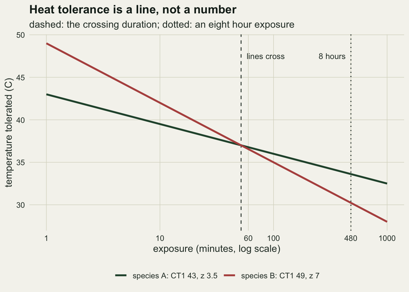
A ramp is a static assay integrated over time
A ramp assay does not hold the temperature still, so it needs one more assumption to be tied to the line: how exposure at one temperature adds to exposure at another. The simplest rule is that damage accumulates additively and is never repaired, the same bookkeeping that Miner’s rule applies to fatigue in materials. At temperature T the animal uses up a fraction 1 / t(T) of its tolerance per minute, and it is knocked down when the fractions sum to one. This is the model, not a tested fact here: heat hardening during a slow ramp, or repair at the cool start, would break it, and nothing below checks either. The direct additivity test of Jorgensen and colleagues moved one species between two static temperatures; separately, they found a good correlation between ramp CTmax predicted from static assays and ramp CTmax measured in Drosophila at three ramping rates, a check of the model’s predictions rather than of hardening or repair as such.
Under that rule a linear ramp from a start temperature T0 at r degrees per minute has a closed form. Changing the variable of integration from time to temperature (dT = r dt) turns the sum into the integral of 10^((T - CT1) / z) / r from T0 to CTmax, which is z / (r ln 10) times the difference of that power at the two ends. Setting it to one gives
CTmax = CT1 + z log10( r ln10 / z + 10^((T0 - CT1) / z) ),
and because the start term is negligible whenever the ramp starts several z below the knockdown temperature, the familiar form is CTmax = CT1 + z log10(r ln10 / z). The logarithm is base 10 because the line is written in base 10, the ln 10 comes from integrating a base 10 power, and r is in degrees per minute because t is in minutes. The same formula can be read backwards: a ramp at rate r knocks the animal down at the temperature it would tolerate for z / (r ln10) minutes of static exposure, so a species with a larger z is, in effect, being tested over a longer exposure at the same ramping rate. The check below integrates damage numerically on a time step of two thousandths of a minute, with the ramp starting at 20 degrees, and compares the knockdown temperature with both forms.
temp_start <- 20
ramp_closed <- function(ct1, z, r) ct1 + z * log10(r * log(10) / z)
ramp_exact  <- function(ct1, z, r, t0 = temp_start)
  ct1 + z * log10(r * log(10) / z + 10^((t0 - ct1) / z))
ramp_numeric <- function(ct1, z, r, t0 = temp_start, dt = 0.002) {
  time_grid <- seq(0, (ct1 + 5 - t0) / r, by = dt)
  temp_grid <- t0 + r * time_grid
  damage    <- cumsum(10^((temp_grid - ct1) / z)) * dt
  k <- which(damage >= 1)[1]
  frac <- (1 - damage[k - 1]) / (damage[k] - damage[k - 1])
  temp_grid[k - 1] + frac * (temp_grid[k] - temp_grid[k - 1])
}

rate_grid <- c(0.05, 0.1, 0.25, 0.5, 1, 2)
ramp_tab <- expand.grid(rate = rate_grid, species = c("A", "B"),
                        stringsAsFactors = FALSE)
ramp_tab$closed  <- ramp_closed(ct1_sp[ramp_tab$species], z_sp[ramp_tab$species], ramp_tab$rate)
ramp_tab$exact   <- ramp_exact(ct1_sp[ramp_tab$species], z_sp[ramp_tab$species], ramp_tab$rate)
ramp_tab$numeric <- mapply(ramp_numeric, ct1_sp[ramp_tab$species],
                           z_sp[ramp_tab$species], ramp_tab$rate)
gap_exact  <- max(abs(ramp_tab$numeric - ramp_tab$exact))
gap_closed <- max(abs(ramp_tab$numeric - ramp_tab$closed))
row_gap    <- ramp_tab[which.max(abs(ramp_tab$numeric - ramp_tab$closed)), ]
stopifnot(which.min((ramp_tab$numeric - temp_start) / z_sp[ramp_tab$species]) ==
          which.max(abs(ramp_tab$numeric - ramp_tab$closed)))

r_use    <- 0.25
ramp_use <- ramp_closed(ct1_sp, z_sp, r_use)
ramp_lead <- unname(ramp_use["B"] - ramp_use["A"])
equiv_min <- z_sp / (r_use * log(10))

u_swap <- (ct1_sp["A"] - ct1_sp["B"] - z_sp["A"] * log10(z_sp["A"]) +
           z_sp["B"] * log10(z_sp["B"])) / (z_sp["B"] - z_sp["A"])
r_swap    <- unname(10^u_swap / log(10))
ramp_swap <- unname(ramp_closed(ct1_sp["A"], z_sp["A"], r_swap))
equiv_swap <- z_sp / (r_swap * log(10))
r_swap_ex <- uniroot(function(r) ramp_exact(ct1_sp[["A"]], z_sp[["A"]], r) -
                       ramp_exact(ct1_sp[["B"]], z_sp[["B"]], r), c(0.01, 1), tol = 1e-10)$root
stopifnot(r_swap_ex < r_swap)

slope_num <- sapply(c("A", "B"), function(s)
  unname(coef(lm(numeric ~ log10(rate), data = ramp_tab[ramp_tab$species == s, ]))[2]))
Across ramping rates from 0.05 to 2 degrees per minute, the numerically integrated knockdown temperature differs from the exact closed form by at most 0.0020 degrees and from the short form by at most 0.013 degrees; the largest short-form gap is for species B at 0.05 degrees per minute, where knockdown comes closest, in units of z, to the 20 degree start.
At the quarter degree per minute of the opening, species A is knocked down at 40.26 degrees and species B at 41.41, so the ramp ranks B ahead by 1.15 degrees. By the backwards reading, the ramp compares A’s line at 6.1 minutes with B’s at 12.2: B is always tested over twice the exposure (the ratio of the z values). Equating the two short ramp formulas gives the rate at which the ranking swaps, again in closed form,
log10(r ln10) = (CT1A - CT1B + zB log10 zB - zA log10 zA) / (zB - zA),
here 0.117 degrees per minute, where both species reach 39.11 degrees (the start term lowers the swap rate by 0.4 per cent); only ramps slower than that rank species A first. At that rate the equivalent exposures are 12.9 and 25.9 minutes, both still short of the 51.8 minute static crossing, which is why the ramp swap cannot be read off the static lines. The ramp formula also says how to get z out of ramps: CTmax rises by z for every tenfold increase in the ramping rate. The slope of the numerically integrated CTmax on log10 of the rate is 3.499 for species A and 6.991 for species B, against z values of 3.5 and 7; the small shortfall for B is the start term at the slow end of the grid.
rate_fine <- 10^seq(log10(0.02), log10(2), length.out = 200)
ramp_line <- rbind(
  data.frame(rate = rate_fine, ctmax = ramp_closed(ct1_sp["A"], z_sp["A"], rate_fine),
             species = "species A: CT1 43, z 3.5"),
  data.frame(rate = rate_fine, ctmax = ramp_closed(ct1_sp["B"], z_sp["B"], rate_fine),
             species = "species B: CT1 49, z 7"))
ramp_pts <- data.frame(rate = ramp_tab$rate, ctmax = ramp_tab$numeric,
                       species = ifelse(ramp_tab$species == "A",
                                        "species A: CT1 43, z 3.5",
                                        "species B: CT1 49, z 7"))

ggplot(ramp_line, aes(rate, ctmax, colour = species)) +
  geom_vline(xintercept = r_swap, linetype = "dashed", colour = te_body, linewidth = 0.5) +
  geom_vline(xintercept = r_use, linetype = "dotted", colour = te_body, linewidth = 0.6) +
  geom_line(linewidth = 1.1) +
  geom_point(data = ramp_pts, size = 2.6, shape = 21, fill = te_paper, stroke = 1) +
  scale_x_log10(breaks = c(0.02, 0.05, 0.1, 0.25, 0.5, 1, 2),
                labels = c("0.02", "0.05", "0.1", "0.25", "0.5", "1", "2")) +
  scale_colour_manual(values = c(te_forest, te_rust), name = NULL) +
  labs(x = "ramping rate (C per minute, log scale)", y = "CTmax at knockdown (C)",
       title = "The ramp chooses the duration",
       subtitle = "lines: closed form; circles: damage integrated numerically") +
  theme_datasheet() +
  theme(legend.position = "bottom")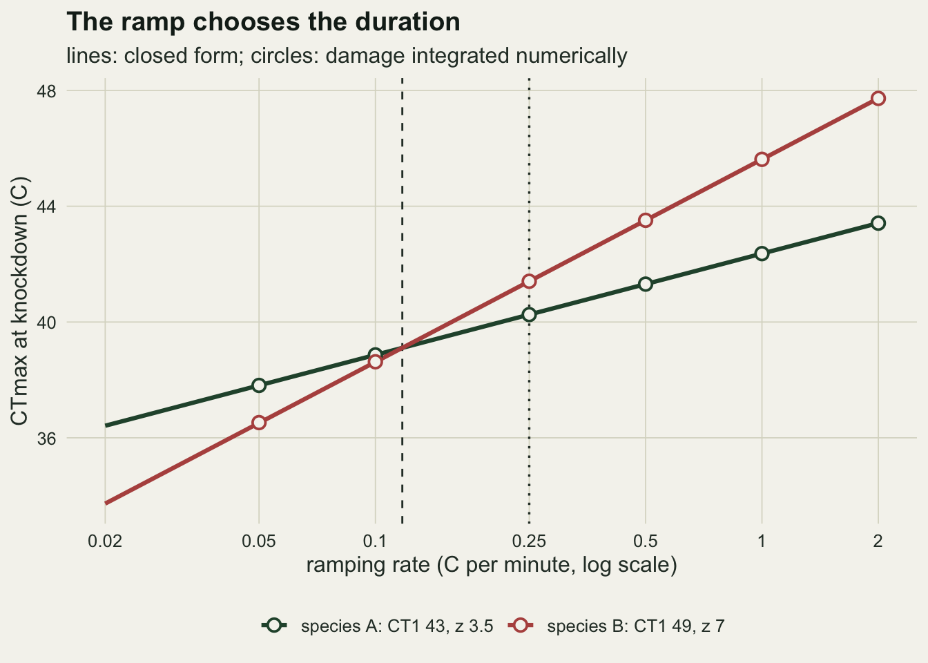
Estimating z from static knockdown assays
Everything above assumed CT1 and z were known. In practice they come from static assays: groups of animals held at several constant temperatures, with the knockdown time of each animal recorded. The design below is fixed before any fit is run. Five temperatures from a lowest temperature up to 43 degrees, equally spaced, with 12 animals at each. Individuals differ only in CT1, with a standard deviation of 0.6 degrees around the species value; their z is the species value. Observation stops after 60 minutes, and an animal still standing then is recorded as surviving to 60 minutes.
Under that model log10 of each animal’s knockdown time is normal with mean (CT1 - T) / z and standard deviation 0.6 / z, so a lognormal accelerated failure time regression is the correct model, not an approximation. In survreg it reads log t = b0 + b1 T + sigma e with natural logarithms, which matches the line when z = -ln10 / b1 and CT1 = -b0 / b1. The default distribution of survreg is the Weibull, so the lognormal has to be asked for; the lognormal family transforms time with the natural log; and the scale sigma is estimated rather than fixed. The chunk checks those three statements against the installed survival package (3.8-6 when this page was built); the default is the same in the current upstream source (survival 3.8-13).
Three ways of handling the animals still standing at 60 minutes are compared. The censored fit keeps them as right-censored observations, which is the likelihood that Values below the detection limit in R builds by hand for non-detects, here with the limit on the other side. Dropping them fits ordinary least squares of log10 time on temperature to the knocked-down animals only. Substituting gives every survivor a knockdown time of exactly 60 minutes and fits the same regression to all animals. A second closed form sets the scale of the design. The median animal lasts exactly the observation time at the temperature CT1 - z log10(60); below it most animals at a temperature are censored, above it most are knocked down.
sd_ct1   <- 0.6
n_animal <- 12
n_temp   <- 5
temp_top <- 43
t_stop   <- 60
temp_half <- unname(ct1_sp["A"] - z_sp["A"] * log10(t_stop))
truth_long <- unname(tol_long["A"])

sim_assay <- function(temps, sd_z = 0, gumbel = FALSE) {
  temp_v <- rep(temps, each = n_animal)
  n_all  <- length(temp_v)
  if (gumbel) {
    g_raw <- -log(rexp(n_all)) + log(log(2))
    log_t <- (ct1_sp[["A"]] - temp_v) / z_sp[["A"]] +
      g_raw / (pi / sqrt(6)) * sd_ct1 / z_sp[["A"]]
  } else {
    ct_i  <- rnorm(n_all, ct1_sp[["A"]], sd_ct1)
    z_i   <- if (sd_z > 0) rnorm(n_all, z_sp[["A"]], sd_z) else z_sp[["A"]]
    log_t <- (ct_i - temp_v) / z_i
  }
  t_kd <- 10^log_t
  data.frame(temp = temp_v, time = pmin(t_kd, t_stop), dead = t_kd < t_stop)
}

fit_three <- function(d) {
  b_c <- coef(survreg(Surv(time, dead) ~ temp, data = d, dist = "lognormal"))
  z_c <- -log(10) / b_c[[2]]; ct_c <- -b_c[[1]] / b_c[[2]]
  b_d <- coef(lm(log10(time) ~ temp, data = d[d$dead, ]))
  z_d <- -1 / b_d[[2]]; ct_d <- -b_d[[1]] / b_d[[2]]
  b_s <- coef(lm(log10(time) ~ temp, data = d))
  z_s <- -1 / b_s[[2]]; ct_s <- -b_s[[1]] / b_s[[2]]
  c(z_cens = z_c, z_drop = z_d, z_sub = z_s,
    p_cens = ct_c - z_c * log10(t_long), p_drop = ct_d - z_d * log10(t_long),
    p_sub = ct_s - z_s * log10(t_long), censored = mean(!d$dead))
}

set.seed(2410)
one_narrow <- sim_assay(seq(39, temp_top, length.out = n_temp))
one_spread <- sim_assay(seq(35, temp_top, length.out = n_temp))
fit_guard  <- survreg(Surv(time, dead) ~ temp, data = one_spread, dist = "lognormal")
stopifnot(identical(eval(formals(survreg)$dist), "weibull"),
          isTRUE(all.equal(survreg.distributions$lognormal$trans(10), log(10))),
          identical(eval(formals(survreg)$scale), 0),
          nrow(vcov(fit_guard)) == 3)
est_narrow <- fit_three(one_narrow)
est_spread <- fit_three(one_spread)
cens_one   <- tapply(!one_spread$dead, one_spread$temp, sum)
stopifnot(cens_one[1] == n_animal, all(one_narrow$dead))
The median animal of species A lasts exactly 60 minutes at 36.78 degrees. The narrow design, 39 to 43 degrees in steps of one degree, sits entirely above that temperature; the spread design, 35 to 43 in steps of two, reaches below it. In the one simulated assay of each shown below, no animal in the narrow design survives the hour, while in the spread design all 12 animals at 35 degrees and 4 at 37 degrees are still standing. On this single draw the censored fit gives z = 3.84 for the spread design, dropping the survivors gives 4.04, and substituting 60 minutes gives 4.60, against a true 3.5. One draw shows the mechanism, not its size; the next section measures that.
pred_lines <- function(d, est_row, lab) {
  temp_seq <- seq(min(d$temp) - 0.5, temp_top + 0.5, length.out = 50)
  z_c <- est_row[["z_cens"]]; z_d <- est_row[["z_drop"]]
  ct_c <- est_row[["p_cens"]] + z_c * log10(t_long)
  ct_d <- est_row[["p_drop"]] + z_d * log10(t_long)
  rbind(data.frame(temp = temp_seq, time = 10^((ct1_sp[["A"]] - temp_seq) / z_sp[["A"]]),
                   line = "true line", design = lab),
        data.frame(temp = temp_seq, time = 10^((ct_c - temp_seq) / z_c),
                   line = "censored fit", design = lab),
        data.frame(temp = temp_seq, time = 10^((ct_d - temp_seq) / z_d),
                   line = "survivors dropped", design = lab))
}
lab_n <- "narrow design: 39 to 43 C"
lab_s <- "spread design: 35 to 43 C"
pts_df <- rbind(cbind(one_narrow, design = lab_n), cbind(one_spread, design = lab_s))
pts_df$status <- ifelse(pts_df$dead, "knocked down", "still standing at 60 min")
line_df <- rbind(pred_lines(one_narrow, est_narrow, lab_n),
                 pred_lines(one_spread, est_spread, lab_s))
line_df$line <- factor(line_df$line, levels = c("true line", "censored fit", "survivors dropped"))

ggplot(pts_df, aes(temp, time)) +
  geom_hline(yintercept = t_stop, colour = te_line, linewidth = 0.8) +
  geom_line(data = line_df, aes(colour = line, linetype = line), linewidth = 0.9) +
  geom_point(aes(shape = status), colour = te_ink, size = 1.9,
             position = position_jitter(width = 0.12, height = 0, seed = 7)) +
  facet_wrap(~ design) +
  scale_y_log10(breaks = c(0.3, 1, 3, 10, 30, 60, 200)) +
  scale_colour_manual(values = c(te_gold, te_forest, te_rust), name = NULL) +
  scale_linetype_manual(values = c("dashed", "solid", "solid"), name = NULL) +
  scale_shape_manual(values = c(16, 2), name = NULL) +
  labs(x = "assay temperature (C)", y = "knockdown time (minutes, log scale)",
       title = "Survivors sit on the stop line",
       subtitle = "grey line: observation stops at 60 minutes") +
  theme_datasheet() +
  theme(legend.position = "bottom", legend.box = "vertical")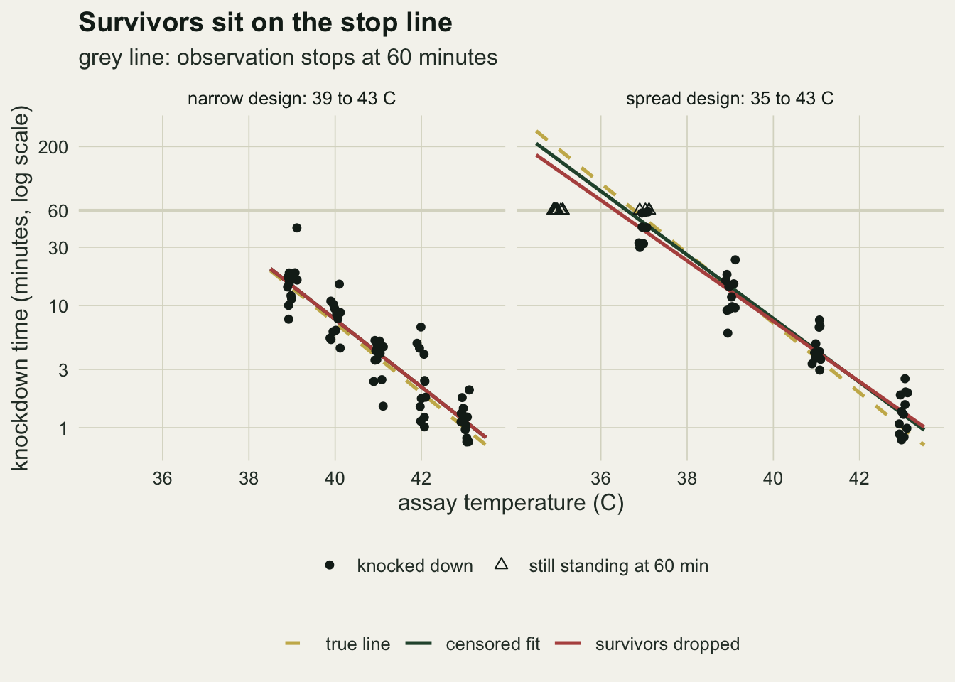
Spreading the temperatures, and what censoring then costs
The quantity a heatwave question needs is the temperature that kills half the animals in eight hours: CT1 - z log10(480) on the true line, 33.62 degrees for species A. Every design predicts it by extrapolation, because no animal is watched for more than an hour, and the error of that prediction is measured on the temperature axis, in degrees, at a fixed duration of 480 minutes. An error in z enters it multiplied by log10(480), so the eight hour prediction is where a biased or noisy z shows. The sweep moves the lowest assay temperature from 39 down to 33 degrees in steps of one degree, always with five equally spaced temperatures up to 43 and 12 animals at each, so every design uses 60 animals. Each design is simulated 1000 times; that number was set before the run so that the Monte Carlo standard error of a mean z is well under a hundredth of a degree.
n_rep    <- 1000
low_grid <- 39:33

set.seed(8124)
sweep_raw <- lapply(low_grid, function(t_low) {
  temps <- seq(t_low, temp_top, length.out = n_temp)
  t(replicate(n_rep, fit_three(sim_assay(temps))))
})
Warning in survreg.fit(X, Y, weights, offset, init = init, controlvals =
control, : Ran out of iterations and did not convergermse_se <- function(err) {
r_val <- sqrt(mean(err^2))
c(rmse = r_val, se = sd(err^2) / sqrt(length(err)) / (2 * r_val))
}
sweep_tab <- do.call(rbind, lapply(seq_along(low_grid), function(i) {
m <- sweep_raw[[i]]
e_c <- m[, "p_cens"] - truth_long
e_d <- m[, "p_drop"] - truth_long
e_s <- m[, "p_sub"] - truth_long
data.frame(t_low = low_grid[i], censored = mean(m[, "censored"]),
z_cens = mean(m[, "z_cens"]), z_drop = mean(m[, "z_drop"]),
z_sub = mean(m[, "z_sub"]),
z_cens_se = sd(m[, "z_cens"]) / sqrt(n_rep),
z_drop_se = sd(m[, "z_drop"]) / sqrt(n_rep),
z_cens_sd = sd(m[, "z_cens"]),
rmse_cens = rmse_se(e_c)[["rmse"]], rmse_cens_se = rmse_se(e_c)[["se"]],
rmse_drop = rmse_se(e_d)[["rmse"]], rmse_drop_se = rmse_se(e_d)[["se"]],
rmse_sub = sqrt(mean(e_s^2)),
bias_cens = mean(e_c), bias_drop = mean(e_d))
}))
stopifnot(all(is.finite(unlist(sweep_raw))))
row_n <- sweep_tab[sweep_tab$t_low == 39, ]
row_s <- sweep_tab[sweep_tab$t_low == 35, ]
cut_pct <- 100 * (1 - row_s$rmse_cens / row_n$rmse_cens)
gap_rmse <- row_n$rmse_cens - row_s$rmse_cens
gap_se <- sqrt(row_n$rmse_cens_se^2 + row_s$rmse_cens_se^2)
drop_bias <- row_s$z_drop - z_sp[["A"]]
m_s <- sweep_raw[[which(low_grid == 35)]]
drop_in_se <- (row_s$z_drop - row_s$z_cens) /
(sd(m_s[, "z_drop"] - m_s[, "z_cens"]) / sqrt(n_rep))
pct_high <- 100 * mean(m_s[, "z_cens"] >= est_spread[["z_cens"]])
row_best <- sweep_tab[which.min(sweep_tab$rmse_cens), ]
z_cens_rng <- range(sweep_tab$z_cens - z_sp[["A"]])
z_se_max <- max(sweep_tab$z_cens_se)
row_low <- sweep_tab[sweep_tab$t_low == min(low_grid), ]
p_cens_at <- function(temp) 1 - pnorm((log10(t_stop) - (ct1_sp[["A"]] - temp) / z_sp[["A"]]) /
(sd_ct1 / z_sp[["A"]]))
temps_35 <- seq(35, temp_top, length.out = n_temp)
temps_33 <- seq(33, temp_top, length.out = n_temp)
cens_35 <- p_cens_at(temps_35)
cens_33 <- p_cens_at(temps_33)
near_best <- sweep_tab$t_low[sweep_tab$rmse_cens - row_best$rmse_cens <=
2 * sqrt(sweep_tab$rmse_cens_se^2 + row_best$rmse_cens_se^2)]Spreading the design helps the prediction. With the narrow design the root mean square error of the eight hour prediction is 0.418 degrees (Monte Carlo standard error 0.010); with the spread design and the censored fit it is 0.261 (standard error 0.006), a cut of 37 per cent and 14 standard errors of the difference. The narrow design censors 0.0 per cent of the animals and the spread design 27.1 per cent. The standard deviation of the censored-fit z falls from 0.195 to 0.137: the cooler temperatures anchor the line nearer to the long exposures it has to reach. The single spread-design draw shown earlier, with a censored-fit z of 3.84, was an unlucky one: only 1.1 per cent of the 1000 censored fits at that design gave a z as high or higher.
The censored fit stays on the true z throughout the sweep: its mean is within 0.010 of 3.5 at every lowest temperature (Monte Carlo standard error at most 0.0062), and its mean eight hour prediction error is -0.002 degrees at the spread design. Dropping the survivors does not. At the spread design it returns a mean z of 3.670, 0.170 above the truth and 73 standard errors of the paired difference away from the censored fit on the same data sets. The animals it drops are the ones that would have lasted longest at the cool temperatures, so the cool end of the line is pulled toward short times and the line of log time against temperature comes out too flat, which is a z too large. Its eight hour prediction is biased by -0.385 degrees, and its root mean square error, 0.477 degrees, is larger than the 0.418 of the narrow design that censors nothing. Spreading the temperatures and then discarding the survivors is worse than not spreading them. Substituting the stop time is worse again, because it pins the cool end of the line at 60 minutes: at the spread design its mean z is 4.30 and its eight hour root mean square error 1.70 degrees, which is why it is left out of the figure below.
The bias from dropping is not a smooth function of the share censored (itself a closed form, one minus the normal probability that an animal’s log10 knockdown time falls below log10(60), averaged over the temperatures: 0.271 for the spread design against 0.271 simulated). It depends on whether some temperature in the design splits its animals at the stop, so that the survivors are a selected tail of the group rather than all of it. In the spread design the group at 37 degrees is censored with probability 0.35 per animal, a group split by the stop. With the lowest temperature at 33 degrees, 40 per cent of the animals are censored, but the two coolest groups, at 33.0 and 35.5 degrees, are censored with probabilities 1.000 and 0.983, and the next, at 38.0, with 0.021: almost nothing is split. Dropping there gives a mean z of 3.558, still above the truth but less so than at 35 degrees. The censored fit does not need to know any of that.
Its own error is smallest with the lowest temperature at 36 degrees (root mean square error 0.250), and the designs within two Monte Carlo standard errors of that minimum have their lowest temperature between 35 and 37 degrees. That is around the 36.78 degrees at which the median animal lasts exactly the hour. Cooler than that, the extra censored animals carry less information and the error rises again, to 0.319 at 33 degrees.
sweep_long <- rbind(
  data.frame(t_low = sweep_tab$t_low, value = sweep_tab$rmse_cens,
             fit = "censored fit", panel = "8 h prediction RMSE (C)"),
  data.frame(t_low = sweep_tab$t_low, value = sweep_tab$rmse_drop,
             fit = "survivors dropped", panel = "8 h prediction RMSE (C)"),
  data.frame(t_low = sweep_tab$t_low, value = sweep_tab$z_cens,
             fit = "censored fit", panel = "mean estimated z"),
  data.frame(t_low = sweep_tab$t_low, value = sweep_tab$z_drop,
             fit = "survivors dropped", panel = "mean estimated z"),
  data.frame(t_low = sweep_tab$t_low, value = sweep_tab$censored,
             fit = "share censored", panel = "share of animals censored"))
sweep_long$panel <- factor(sweep_long$panel,
  levels = c("8 h prediction RMSE (C)", "mean estimated z", "share of animals censored"))
ref_df <- data.frame(panel = factor("mean estimated z", levels = levels(sweep_long$panel)),
                     value = z_sp[["A"]])

ggplot(sweep_long, aes(t_low, value, colour = fit)) +
  geom_hline(data = ref_df, aes(yintercept = value), linetype = "dashed", colour = te_body, linewidth = 0.5) +
  geom_line(linewidth = 0.9) +
  geom_point(size = 2.2) +
  facet_wrap(~ panel, ncol = 1, scales = "free_y") +
  scale_x_continuous(breaks = low_grid) +
  scale_colour_manual(values = c("censored fit" = te_forest,
                                 "survivors dropped" = te_rust,
                                 "share censored" = te_gold), name = NULL) +
  labs(x = "lowest assay temperature (C); five temperatures up to 43 C",
       y = NULL, title = "Spread the assay, keep the survivors",
       subtitle = "dashed: the true z of 3.5; 1000 simulated assays per design") +
  theme_datasheet() +
  theme(legend.position = "bottom")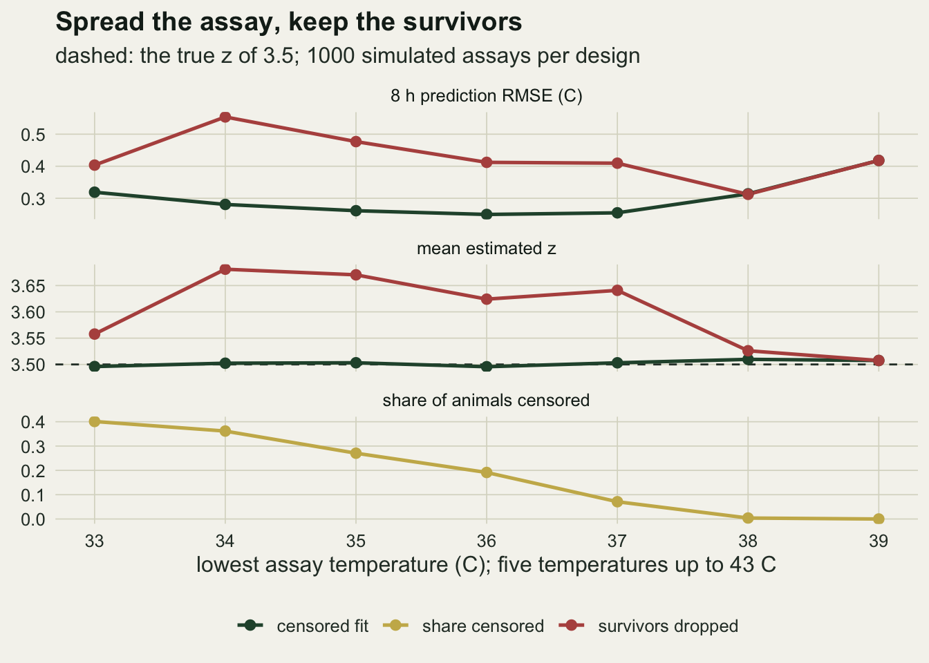
When the animals differ in more than CT1
The censored lognormal fit is unbiased above because it is the exact model for the simulated animals. Two departures are cheap to test. In the first, individuals also differ in z, drawn from a normal distribution around 3.5 with a standard deviation of 0.35 or 0.7, independently of CT1. An animal’s tolerance at any duration is linear in its CT1 and z, so the median animal still lies exactly on the species line, and the target of 3.5 for z and 33.62 degrees at eight hours does not move. What changes is log time at a given temperature, (CT1 - T) / z with both drawn per animal: it is skewed, and its spread grows with the distance from CT1. Its median stays on the line but its mean does not, because the average of 1 / z over the animals exceeds 1 / 3.5. A lognormal fit treats mean and median as the same, and without censoring it is least squares on log time, which follows the mean line; censoring at the stop hides the long tail from the fit, and the direction of the bias then depends on the design, as the runs below show. In the second, the scatter of log time around the line is a skewed Gumbel distribution with its median on the line and the same standard deviation as before, so the lognormal family is wrong but the scale is constant.
n_rep_mis <- 1000
mis_cells <- expand.grid(case = c("z sd 0.35", "z sd 0.7", "Gumbel scatter"),
                         t_low = c(39, 35), stringsAsFactors = FALSE)
set.seed(5117)
mis_tab <- do.call(rbind, lapply(seq_len(nrow(mis_cells)), function(i) {
  temps <- seq(mis_cells$t_low[i], temp_top, length.out = n_temp)
  sd_z  <- switch(mis_cells$case[i], "z sd 0.35" = 0.35, "z sd 0.7" = 0.7, 0)
  m <- t(replicate(n_rep_mis, fit_three(sim_assay(temps, sd_z = sd_z,
                                                    gumbel = mis_cells$case[i] == "Gumbel scatter"))))
  e_c <- m[, "p_cens"] - truth_long
  data.frame(case = mis_cells$case[i], t_low = mis_cells$t_low[i],
             z_bias = mean(m[, "z_cens"]) - z_sp[["A"]],
             z_se = sd(m[, "z_cens"]) / sqrt(n_rep_mis),
             bias = mean(e_c), bias_se = sd(e_c) / sqrt(n_rep_mis),
             rmse = sqrt(mean(e_c^2)), censored = mean(m[, "censored"]),
             rmse_drop = sqrt(mean((m[, "p_drop"] - truth_long)^2)))
}))
Warning in survreg.fit(X, Y, weights, offset, init = init, controlvals =
control, : Ran out of iterations and did not convergez_mean_line <- 1 / mean(1 / rnorm(1e6, z_sp[["A"]], 0.7))
shift_mean_line <- (z_sp[["A"]] - z_mean_line) * log10(t_long)
base_rows <- data.frame(case = "CT1 only", t_low = c(39, 35),
z_bias = c(row_n$z_cens, row_s$z_cens) - z_sp[["A"]],
z_se = c(row_n$z_cens_se, row_s$z_cens_se),
bias = c(row_n$bias_cens, row_s$bias_cens),
bias_se = c(sd(sweep_raw[[1]][, "p_cens"]),
sd(sweep_raw[[5]][, "p_cens"])) / sqrt(n_rep),
rmse = c(row_n$rmse_cens, row_s$rmse_cens),
censored = c(row_n$censored, row_s$censored),
rmse_drop = c(row_n$rmse_drop, row_s$rmse_drop))
stopifnot(sweep_tab$t_low[c(1, 5)] == c(39, 35))
mis_all <- rbind(base_rows, mis_tab)
mis_get <- function(cs, tl, col) mis_all[mis_all$case == cs & mis_all$t_low == tl, col]
stopifnot(mis_get("z sd 0.7", 39, "bias") > 0, mis_get("z sd 0.7", 35, "bias") < 0,
mis_get("z sd 0.7", 39, "rmse_drop") < mis_get("z sd 0.7", 39, "rmse"),
mis_get("z sd 0.7", 35, "rmse_drop") > mis_get("z sd 0.7", 35, "rmse"),
mis_get("z sd 0.7", 35, "rmse") < mis_get("z sd 0.7", 39, "rmse"),
mis_get("z sd 0.7", 39, "z_bias") < 0, mis_get("z sd 0.7", 35, "z_bias") > 0,
shift_mean_line > 0)
gum_gap <- sd_ct1 * (-digamma(1) + log(log(2))) / (pi / sqrt(6))
gum_bias <- c(mis_get("Gumbel scatter", 39, "bias"), mis_get("Gumbel scatter", 35, "bias"))
stopifnot(all(gum_bias > 0), all(gum_bias < gum_gap))With a z standard deviation of 0.35 the censored fit’s eight hour prediction is off by +0.062 degrees in the narrow design and -0.065 in the spread design (Monte Carlo standard errors 0.015 and 0.010). With 0.7 the biases are +0.295 and -0.261 degrees, and the mean z is off by -0.104 and +0.150, in opposite directions for the two designs. Averaged over a million simulated animals, 1 / z gives a mean line with the slope of a z of 3.35, which would move the eight hour prediction up by 0.41 degrees; the narrow design, which censors 1.2 per cent of the animals here, is biased in that direction, and the spread design, which censors 27.8 per cent, in the other. So the statement that the censored fit keeps z unbiased holds for animals that differ only in CT1; once z varies between individuals, the censored lognormal fit is biased too, by an amount that depends on the design. The root mean square errors in that case are 0.646 and 0.516 degrees, so the spread design is still the better of the two. Dropping the survivors gives 0.566 in the narrow design, below the censored fit, and 1.414 in the spread design, far above it.
The Gumbel scatter moves z by +0.016 and +0.021 but the eight hour prediction by +0.070 and +0.055 degrees, in the direction of the skew: the scatter’s mean lies 0.099 degrees above its median on the temperature axis, and the lognormal fit treats the two as the same. Both biases are positive and smaller than that gap.
mis_all$design <- ifelse(mis_all$t_low == 39, "narrow: 39 to 43 C", "spread: 35 to 43 C")
mis_all$case <- factor(mis_all$case,
                       levels = rev(c("CT1 only", "z sd 0.35", "z sd 0.7", "Gumbel scatter")))

ggplot(mis_all, aes(bias, case, colour = design)) +
  geom_vline(xintercept = 0, linetype = "dashed", colour = te_body, linewidth = 0.5) +
  geom_errorbar(aes(xmin = bias - 2 * bias_se, xmax = bias + 2 * bias_se),
                orientation = "y", width = 0.2, linewidth = 0.6,
                position = position_dodge(width = 0.5)) +
  geom_point(size = 2.6, position = position_dodge(width = 0.5)) +
  scale_colour_manual(values = c(te_gold, te_forest), name = NULL) +
  labs(x = "mean error of the 8 h prediction, censored fit (C)", y = NULL,
       title = "The censored fit is exact only for the model it assumes",
       subtitle = "bars: two Monte Carlo standard errors; 1000 simulated assays per cell") +
  theme_datasheet() +
  theme(legend.position = "bottom")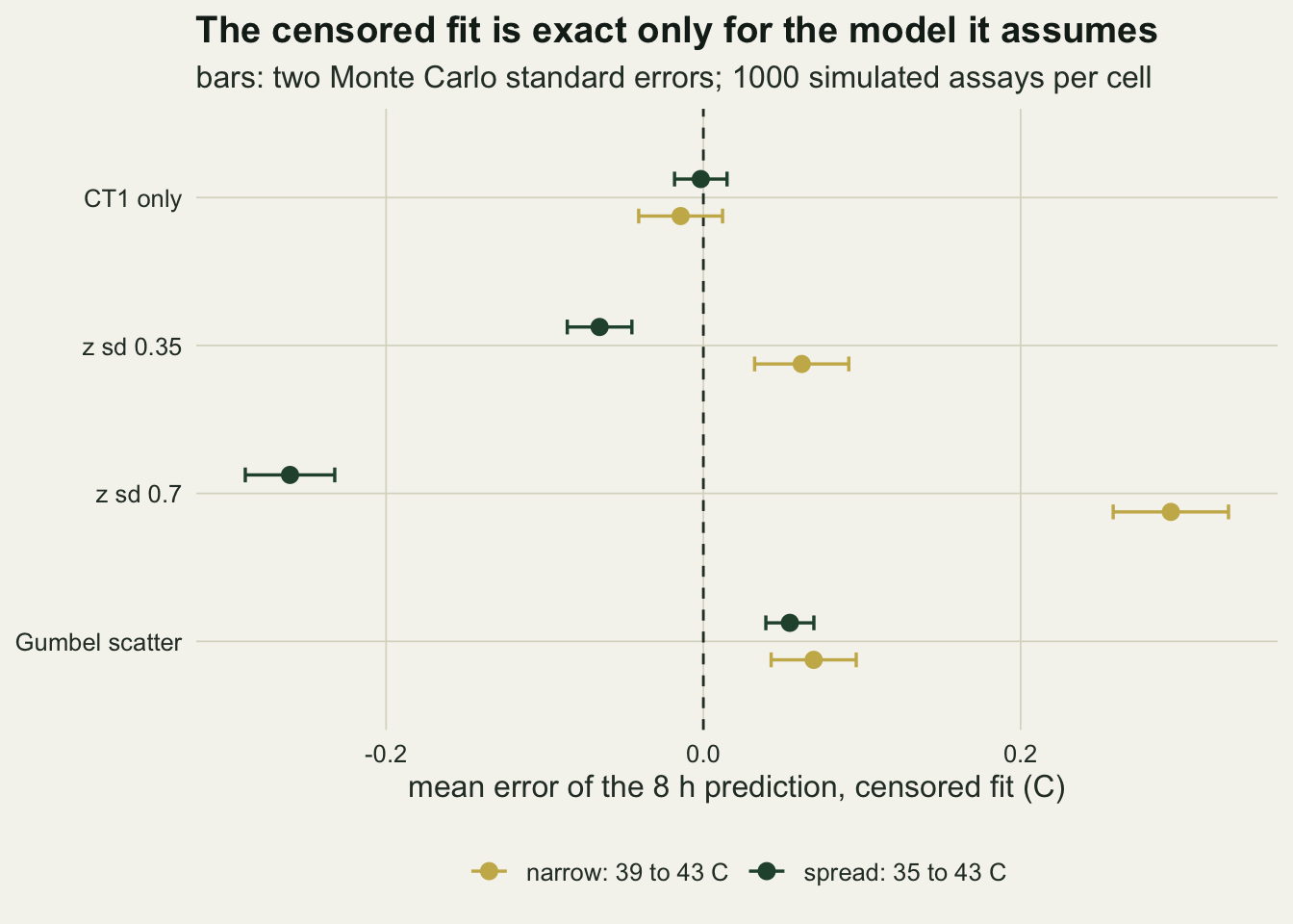
What to report
Report every ramp CTmax with its ramping rate and its start temperature, and do not rank species on ramp CTmax measured at different rates. Under the additive damage model a ramp at r degrees per minute measures the tolerance for z / (r ln10) minutes, which differs between species with different z even at the same rate. If CTmax is available at two or more ramping rates, its slope on log10 of the rate estimates z directly.
For static assays, report the stop time and the number of animals still standing at it for each temperature, and fit the knockdown times with a censored likelihood. In R that is survreg(Surv(time, dead) ~ temp, dist = "lognormal"), with dist given explicitly because the default is the Weibull; z is -ln10 divided by the temperature coefficient and CT1 is minus the intercept divided by it. Do not drop the survivors and do not give them the stop time. Both are ways of throwing away the part of the design that made it worth spreading. The censored lognormal fit is exact only if the animals share z; with a z standard deviation of 0.7 it was off at eight hours by 0.295 degrees in the narrow design and 0.261 in the spread design, in opposite directions (dropping the survivors was still far worse at the spread design), so quote a long exposure tolerance as conditional on that model.
Plan the temperatures with a rough CT1 and z from a pilot. In the sweep above, which used a single stop time, the lowest temperature was most useful near the one at which the median animal lasts the observation time, CT1 - z log10(60), and much cooler temperatures mostly produced survivors. Whether that rule carries over to other stop times was not simulated; with another stop time, noise level or group size the best spread will differ, and the same simulation, run with the pilot values, is a cheap way to look for it. Quote any long exposure tolerance as a temperature at a stated duration, and say how far beyond the longest observation it extrapolates: here an eight hour prediction from animals watched for one hour.
Honest limits
Additive damage without repair is the whole link between the static line and the ramp. Heat hardening during a slow ramp, repair during the cool part of a fluctuating exposure, or a damage rate that changes with accumulated damage would all move the ramp CTmax away from the formula, and the post tests none of them. Nothing here says anything about mortality in the field, where exposure is not a clean ramp and body temperature is not water bath temperature; the simulation assumes that the animal’s temperature follows the set temperature without lag, which is least true at fast ramps and for large animals.
The two species are illustrative constants. The crossing duration and the swap rate are closed forms of those constants and carry no generality beyond them; for another pair of species the lines may cross at seconds, at days or not at all. No sampling noise was put into the ramp CTmax, so nothing is said about how often a real ramp assay of a dozen animals would get the ranking wrong. The assay design has one noise level (a CT1 standard deviation of 0.6 degrees), one stop time, five temperatures and 12 animals each. The best lowest temperature in the sweep depends on all of them, and a longer stop time would change the trade-off by making fewer animals censored at every temperature. The eight hour target is an extrapolation of the line by a factor of eight in time; whether the line stays straight that far is an empirical question for the species at hand, and a curved thermal death time relation would add bias that no design choice here can see.
Knockdown is treated as the endpoint and as the same event at every temperature. In practice knockdown, coma and death can separate at long, mild exposures, and an assay that scores a different event at the cool temperatures builds a bias into z of its own. The departures from the model were two: individual variation in z, independent of CT1, which at a standard deviation of 0.7 moved the eight hour prediction by up to 0.295 degrees, and one skewed error family. Correlated variation in CT1 and z, a mixture of hardened and naive animals, or a hazard that is not a function of the current temperature alone were not simulated.
References
Bigelow WD 1921 Journal of Infectious Diseases 29(5):528-536 (10.1093/infdis/29.5.528)
Rezende EL, Castaneda LE, Santos M 2014 Functional Ecology 28(4):799-809 (10.1111/1365-2435.12268)
Terblanche JS, Deere JA, Clusella-Trullas S, Janion C, Chown SL 2007 Proceedings of the Royal Society B 274(1628):2935-2943 (10.1098/rspb.2007.0985)
Jorgensen LB, Malte H, Orsted M, Klahn NA, Overgaard J 2021 Scientific Reports 11:12840 (10.1038/s41598-021-92004-6)