library(ggplot2)
library(patchwork)
library(survival)

te_paper  <- "#f5f4ee"
te_ink    <- "#16241d"
te_body   <- "#2c3a31"
te_forest <- "#275139"
te_rust   <- "#b5534e"
te_gold   <- "#c9b458"
te_line   <- "#dad9ca"

f3 <- function(x) sprintf("%.3f", round(x, 3))   # matches the printed round(, 3) tables

theme_datasheet <- function() {
  theme_minimal(base_size = 12) +
    theme(plot.background  = element_rect(fill = te_paper, colour = NA),
          panel.background = element_rect(fill = te_paper, colour = NA),
          panel.grid.major = element_line(colour = te_line, linewidth = 0.3),
          panel.grid.minor = element_blank(),
          text             = element_text(colour = te_body),
          plot.title       = element_text(colour = te_ink, face = "bold"),
          plot.subtitle    = element_text(colour = te_body),
          axis.text        = element_text(colour = te_body),
          strip.text       = element_text(colour = te_ink))
}Germination trials as time-to-event data
R
seed ecology
survival analysis
censoring
simulation
ecology tutorial
A slower seed lot reads as less viable when only the final count is tested. Fitting germination trials as interval-censored data with a cure fraction in R.
A restoration nursery has two seed lots of the same grassland forb, one collected on a dry south slope and one from a wet meadow. Each lot goes into the germination cabinet as four Petri dishes of twenty-five seeds, the dishes are checked every morning, and a seed counts as germinated when its radicle shows. After fourteen days the trial stops, the counts are added up, and the lab sheet reports a final germination percentage per lot. The two percentages are compared with a two-proportion test, and the lot with the lower percentage is recorded as the less viable one and sown at a higher rate.
The daily checks hold more than the final count. Each germinated seed has a day on which it was first seen with a radicle, which means it germinated at some time since the previous check: an interval, not a date. Each seed that has not germinated by day fourteen is censored at the end of the trial. And some of those censored seeds never would have germinated, however long the trial ran, because they are dead or deeply dormant. A germination trial is therefore interval-censored time-to-event data with a fraction that never has the event. Two different things can lower a fourteen-day percentage: fewer seeds able to germinate, or the same seeds germinating more slowly so that part of the curve falls after the trial has stopped. The final count cannot tell these apart. A likelihood that carries both a germinable fraction and a time-to-germination distribution can.
None of this is new. Onofri, Gresta and Tei (2010) and Ritz, Pipper and Streibig (2013) argued that germination counts should be analysed as time-to-event data rather than by fitting a curve to the running totals, McNair, Sunkara and Frobish (2012) wrote a practical guide to the non-parametric and semi-parametric time-to-event methods for seed scientists, and Onofri and colleagues (2011) fitted the cure model of Farewell (1982) to germination directly. This post is a demonstration of those arguments in base R, with the rates measured over simulated trials rather than asserted.
Several posts on this site sit next to it. Latency tests when some animals never respond fits a mixture cure model of the same form, with exponential latencies, to behavioural latencies with a hard cap, and shows there that the usual tests fold a change in the share of responders and a change in their speed into one hazard ratio, and how the incidence test loses power as the cap cuts into the responders. Here the events are only known to the day, so the likelihood is interval-censored, and the new parts are what the final-count test of the seed lab does with a slow lot, how the everyday seed summaries drift with trial length, and what a curve fitted to running totals does to the interval. Estimating R0 from incidence data already shows, in its section on cumulative counts, that fitting a model to running totals returns an interval far too narrow; the same trap sits in the seed lab, and it appears here as the second part, not the first, because the parameter that matters more in a germination trial is the one a cumulative curve handles badly: the seeds that never germinate. Interval-censored survival from visit data builds the interval likelihood for radio-tracked birds, where every bird can die; here a share of the seeds cannot germinate at all, which adds one parameter to the same likelihood. Dose-response curves and the LC50 uses the same log-logistic curve on a dose axis with independent animals at each dose; on a time axis the points on a cumulative curve are not independent, because each running total contains the one before it.
A germination trial is a table of intervals
The simulated trial has 100 seeds. Each seed is germinable with probability d, and a germinable seed germinates at a log-logistic time with median t50 of 8 days and slope 4, a curve that germination software commonly fits. Checks are daily, so a seed first seen on day k germinated in the interval from day k - 1 to day k. The trial stops at day 14, 21 or 28. All of these constants, and the replicate counts used below, were fixed before any simulation was run.
The likelihood has one term per check interval and one for the seeds still ungerminated at the end. The probability of germinating in interval k is d times the increase of the log-logistic distribution function over that interval, and the probability of being ungerminated at the end of a trial of length T is 1 - d F(T): a seed is either not germinable, or germinable and slow. The parameters are fitted on the logit scale for d and the log scale for t50 and slope, so optim works without bounds.
n_seed  <- 100
t50_set <- 8
b_set   <- 4
d_set   <- 0.8

F_ll <- function(tt, t50, b) 1 / (1 + (t50 / tt)^b)   # F_ll(0) is 0

sim_counts <- function(n_seed, d, t50, b, t_end) {
  u_time <- runif(n_seed)
  t_germ <- t50 * (u_time / (1 - u_time))^(1 / b)
  day <- ifelse(runif(n_seed) < d, ceiling(t_germ), Inf)
  tabulate(day[day <= t_end], t_end)
}

loglik_cure <- function(cnt, d, t50, b, n_seed) {
  t_end <- length(cnt)
  cum_p <- d * F_ll(0:t_end, t50, b)
  sum(cnt * log(pmax(diff(cum_p), 1e-300))) +
    (n_seed - sum(cnt)) * log(max(1 - cum_p[t_end + 1], 1e-300))
}
nll_cure <- function(par, cnt, n_seed)
  -loglik_cure(cnt, plogis(par[1]), exp(par[2]), exp(par[3]), n_seed)

fit_cure <- function(cnt, n_seed) {
  p_fin <- min(max(sum(cnt) / n_seed, 0.05), 0.94)
  half_day <- which(cumsum(cnt) >= sum(cnt) / 2)[1]
  start_par <- c(qlogis(p_fin + 0.05), log(max(half_day, 1)), log(3))
  opt <- optim(start_par, nll_cure, cnt = cnt, n_seed = n_seed, method = "BFGS",
               hessian = TRUE, control = list(maxit = 500))
  vc <- tryCatch(solve(opt$hessian), error = function(e) matrix(NA, 3, 3))
  list(par = opt$par, se = suppressWarnings(sqrt(diag(vc))),
       nll = opt$value, conv = opt$convergence)
}

set.seed(1512)
cnt_fast <- sim_counts(n_seed, d_set, t50_set, b_set, 21)
cnt_slow <- sim_counts(n_seed, d_set, 12, b_set, 21)
fit_fast <- fit_cure(cnt_fast, n_seed)
fit_slow <- fit_cure(cnt_slow, n_seed)
ex_tab <- rbind(fast = c(final_14 = sum(cnt_fast[1:14]), final_21 = sum(cnt_fast),
                         d_hat = plogis(fit_fast$par[1]), t50_hat = exp(fit_fast$par[2])),
                slow = c(sum(cnt_slow[1:14]), sum(cnt_slow),
                         plogis(fit_slow$par[1]), exp(fit_slow$par[2])))
round(ex_tab, 3)
final_14 final_21 d_hat t50_hat
fast 76 84 0.854 8.096
slow 57 73 0.765 11.528The chunk also draws one pair of lots for a 21-day trial: the lot above, and a second lot identical in every way except that its median germination time is 12 days instead of 8. The fast lot had 76 seeds germinated by day 14 and 84 by day 21; the slow lot had 57 and 73. Fitted on all 21 days, the cure model puts the germinable fraction at 0.854 for the fast lot and 0.765 for the slow one, with medians of 8.10 and 11.53 days.
curve_fit <- function(fit, lab) {
  tt <- seq(0.2, 21, by = 0.1)
  data.frame(day = tt, lot = lab,
             p = plogis(fit$par[1]) * F_ll(tt, exp(fit$par[2]), exp(fit$par[3])))
}
pts <- rbind(data.frame(day = 1:21, p = cumsum(cnt_fast) / n_seed, lot = "median 8 days"),
             data.frame(day = 1:21, p = cumsum(cnt_slow) / n_seed, lot = "median 12 days"))
lines_fit <- rbind(curve_fit(fit_fast, "median 8 days"), curve_fit(fit_slow, "median 12 days"))
ggplot(pts, aes(day, p, colour = lot)) +
  geom_hline(yintercept = d_set, colour = te_body, linetype = "dotted", linewidth = 0.5) +
  geom_vline(xintercept = 14, colour = te_ink, linetype = "dashed", linewidth = 0.6) +
  geom_line(data = lines_fit, linewidth = 0.9) +
  geom_point(size = 2) +
  scale_colour_manual(values = c("median 8 days" = te_forest, "median 12 days" = te_rust), name = NULL) +
  scale_y_continuous(limits = c(0, 1)) +
  labs(x = "day of trial", y = "proportion of seeds germinated",
       title = "Same germinable fraction, different speed",
       subtitle = "dotted line: true germinable fraction 0.8; dashed line: a 14-day trial stops here") +
  theme_datasheet() + theme(legend.position = "bottom")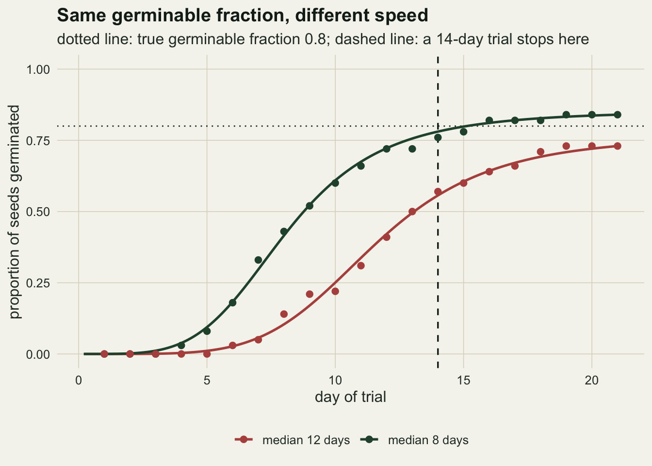
Slower is read as less viable
Now repeat the pair many times. The two lots have the same germinable fraction, 0.8, and differ only in speed. The final-count test is prop.test on the numbers germinated at the end of the trial. The event-time tests are likelihood ratio tests from the cure model fitted to both lots: one for a difference in d, with the medians and slopes left free in each lot, and one for a difference in t50, with d and the slopes left free. A third scenario is the control the other way round: the same speed in both lots and a real difference in germinable fraction, 0.8 against 0.6.
The rejection rate of the final-count test does not need a simulation. The number germinated in each lot is binomial with probability d F(T), so the probability that prop.test rejects is a finite sum over the two binomial distributions. The chunk computes that sum next to the simulated rate.
fit_pair <- function(ca, cb, n_seed) {
  fa <- fit_cure(ca, n_seed); fb <- fit_cure(cb, n_seed)
  nll_full <- fa$nll + fb$nll
  nll_same_d <- function(q) -(loglik_cure(ca, plogis(q[1]), exp(q[2]), exp(q[3]), n_seed) +
                                loglik_cure(cb, plogis(q[1]), exp(q[4]), exp(q[5]), n_seed))
  nll_same_t <- function(q) -(loglik_cure(ca, plogis(q[1]), exp(q[3]), exp(q[4]), n_seed) +
                                loglik_cure(cb, plogis(q[2]), exp(q[3]), exp(q[5]), n_seed))
  o_d <- optim(c(mean(c(fa$par[1], fb$par[1])), fa$par[2:3], fb$par[2:3]), nll_same_d,
               method = "BFGS", control = list(maxit = 1000))
  o_t <- optim(c(fa$par[1], fb$par[1], mean(c(fa$par[2], fb$par[2])), fa$par[3], fb$par[3]),
               nll_same_t, method = "BFGS", control = list(maxit = 1000))
  c(prop = prop.test(c(sum(ca), sum(cb)), c(n_seed, n_seed))$p.value < 0.05,
    lrt_d = 2 * (o_d$value - nll_full) > qchisq(0.95, 1),
    lrt_t50 = 2 * (o_t$value - nll_full) > qchisq(0.95, 1),
    conv = fa$conv + fb$conv + o_d$convergence + o_t$convergence)
}

exact_prop_reject <- function(p_a, p_b, n_seed) {
  xa <- 0:n_seed; wa <- dbinom(xa, n_seed, p_a); wb <- dbinom(xa, n_seed, p_b)
  keep_a <- xa[wa > 1e-9]; keep_b <- xa[wb > 1e-9]
  grid_ab <- expand.grid(a = keep_a, b = keep_b)
  rej <- mapply(function(a, b) suppressWarnings(
    prop.test(c(a, b), c(n_seed, n_seed))$p.value < 0.05), grid_ab$a, grid_ab$b)
  sum(rej * wa[grid_ab$a + 1] * wb[grid_ab$b + 1])
}

n_pair <- 400
scen <- data.frame(scenario = c("speed only", "speed only", "viability only", "viability only, both lots slow"),
                   t_end = c(14, 21, 14, 14), t50_a = c(8, 8, 8, 12),
                   d_b = c(0.8, 0.8, 0.6, 0.6), t50_b = c(12, 12, 8, 12))
set.seed(2604)
pair_res <- lapply(seq_len(nrow(scen)), function(i) {
  runs <- t(replicate(n_pair, suppressWarnings(fit_pair(
    sim_counts(n_seed, d_set, scen$t50_a[i], b_set, scen$t_end[i]),
    sim_counts(n_seed, scen$d_b[i], scen$t50_b[i], b_set, scen$t_end[i]), n_seed))))
  c(colMeans(runs[, 1:3]), conv_bad = sum(runs[, 4] != 0))
})
scen <- cbind(scen, do.call(rbind, pair_res))
scen$p_fin_a <- d_set * F_ll(scen$t_end, scen$t50_a, b_set)
scen$p_fin_b <- scen$d_b * F_ll(scen$t_end, scen$t50_b, b_set)
scen$prop_exact <- mapply(exact_prop_reject, scen$p_fin_a, scen$p_fin_b, MoreArgs = list(n_seed = n_seed))
mcse_pair <- function(p) sqrt(p * (1 - p) / n_pair)
prop_exact_28 <- exact_prop_reject(d_set * F_ll(28, 8, 4), d_set * F_ll(28, 12, 4), n_seed)
round(scen[, -1], 3)
t_end t50_a d_b t50_b prop lrt_d lrt_t50 conv_bad p_fin_a p_fin_b prop_exact
1 14 8 0.8 12 0.850 0.038 0.873 0 0.723 0.520 0.811
2 21 8 0.8 12 0.160 0.065 1.000 0 0.783 0.723 0.130
3 14 8 0.6 8 0.713 0.510 0.050 0 0.723 0.542 0.710
4 14 12 0.6 12 0.428 0.098 0.050 0 0.520 0.390 0.416s14 <- scen[1, ]; s21 <- scen[2, ]; sv <- scen[3, ]; svs <- scen[4, ]
mcse_lo <- mcse_pair(0.05); mcse_hi <- mcse_pair(0.5)
gap_mcse <- (s14$prop - s14$prop_exact) / mcse_pair(s14$prop_exact)In the speed-only scenario at 14 days the expected final proportions are 0.723 for the fast lot and 0.520 for the slow one, although both lots hold the same share of germinable seeds. The exact probability that prop.test declares a difference is 0.811, and the simulation gave 0.850 over 400 pairs. The two differ by 2.0 Monte Carlo standard errors, a high draw rather than a disagreement: the exact value needs no simulation and is the number to use. Four times out of five, then, a lab that compares final percentages after 14 days writes down that the slow lot is less viable.
The likelihood ratio test for a difference in d, on the same pairs, rejected in 0.038 of them, which is within two Monte Carlo standard errors of the 5 per cent level it should hold when d is equal (one standard error is 0.011). The test for a difference in t50 rejected in 0.873. The cure model puts the difference in speed where it is; whether it could also have detected a real difference in d on a lot this slow is the question of the section on plateaus below.
Letting the trial run to 21 days removes most of the confusion without any model, because the slow lot has then germinated most of what it will: the exact rejection rate of the final-count test drops to 0.130 (simulated 0.160), and at 28 days to 0.044. The d test gave 0.065 at 21 days and the t50 test rejected in 1.000 of pairs.
The control scenario shows the price. When the lots really differ in germinable fraction and not in speed, the final-count test rejects in 0.713 of pairs (exact 0.710), and the cure-model test for d in only 0.510. The final-count test is more powerful here because it silently assumes the two lots have the same speed, and in this scenario that assumption happens to be true. The cure model spends information estimating two speeds, and on a 14-day trial with 100 seeds per lot that costs a lot of power. The t50 test stayed at 0.050. Across the 1600 pairs of the four scenarios (the fourth is used further down), 0 reported a convergence failure in any of their four optimisations.
rate_long <- data.frame(
  scenario = rep(paste0(scen$scenario, ", ", scen$t_end, "-day trial"), 3),
  test = rep(c("final count (prop.test)", "cure model: d differs", "cure model: t50 differs"), each = nrow(scen)),
  rate = c(scen$prop, scen$lrt_d, scen$lrt_t50))
rate_long$scenario <- factor(rate_long$scenario, levels = unique(rate_long$scenario))
rate_long$test <- factor(rate_long$test, levels = unique(rate_long$test))
rate_long$lo <- pmax(0, rate_long$rate - 2 * mcse_pair(rate_long$rate))
rate_long$hi <- pmin(1, rate_long$rate + 2 * mcse_pair(rate_long$rate))
exact_pts <- data.frame(scenario = levels(rate_long$scenario), rate = scen$prop_exact,
                        test = factor("final count (prop.test)", levels = levels(rate_long$test)))
ggplot(rate_long, aes(rate, test, colour = test)) +
  geom_vline(xintercept = 0.05, colour = te_ink, linetype = "dashed", linewidth = 0.5) +
  geom_errorbar(aes(xmin = lo, xmax = hi), orientation = "y", width = 0.25, linewidth = 0.6) +
  geom_point(size = 2.8) +
  geom_point(data = exact_pts, shape = 5, size = 4, colour = te_ink) +
  facet_wrap(~ scenario, ncol = 1) +
  scale_colour_manual(values = c(te_rust, te_forest, te_gold), guide = "none") +
  scale_x_continuous(limits = c(0, 1)) +
  labs(x = "proportion of simulated pairs rejected at the 5 per cent level", y = NULL,
       title = "The final count cannot tell slower from less viable",
       subtitle = "dashed line: the 5 per cent level") +
  theme_datasheet()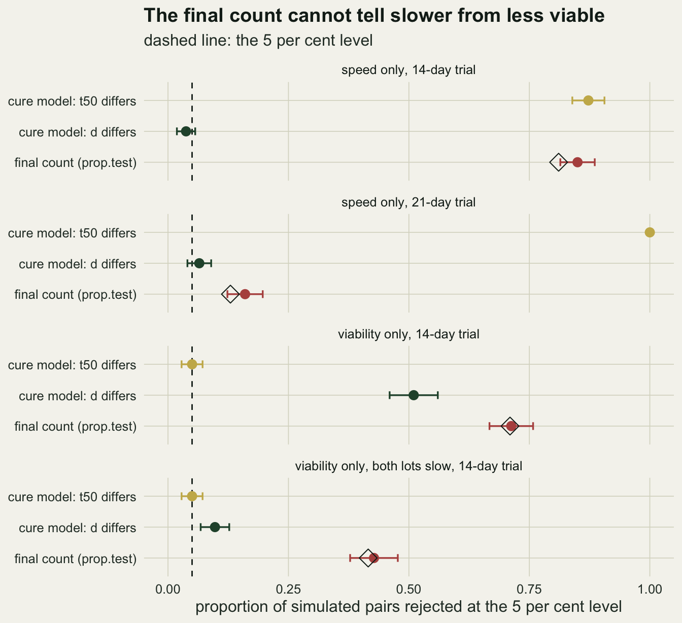
The everyday summaries move with the trial length
Mean germination time is the average day of germination among the seeds that germinated. Because a seed only enters it if it germinated before the trial stopped, it is a truncated mean, and its expected value for daily checks is a short sum: the day k weighted by the probability of germinating on day k, divided by F(T). The germinable fraction cancels. The same truncation affects a survival fit that ignores the non-germinable seeds: survreg with an interval-censored log-logistic, treating every ungerminated seed as merely late, has to stretch its time distribution to account for them.
mgt_exact <- function(t_end, t50, b) {
  k <- 1:t_end; pk <- diff(F_ll(0:t_end, t50, b)); sum(k * pk) / sum(pk)
}
mgt_limit <- mgt_exact(5000, t50_set, b_set)
mean_cont <- t50_set * (pi / b_set) / sin(pi / b_set)

fit_nls <- function(cnt, n_seed) {
  dd <- data.frame(day = seq_along(cnt), p = cumsum(cnt) / n_seed)
  half_day <- which(dd$p >= max(dd$p) / 2)[1]
  m <- tryCatch(nls(p ~ dmax / (1 + (t50 / day)^b), data = dd,
                    start = list(dmax = max(dd$p) + 0.01, t50 = half_day, b = 3)),
                error = function(e) NULL)
  if (is.null(m)) return(rep(NA_real_, 4))
  s <- summary(m)$coefficients
  unname(c(s["t50", 1:2], s["dmax", 1:2]))
}
fit_survreg <- function(cnt, n_seed) {
  t_end <- length(cnt); day <- rep(seq_len(t_end), cnt); n_left <- n_seed - sum(cnt)
  lo <- c(ifelse(day == 1, NA, day - 1), rep(t_end, n_left))
  hi <- c(day, rep(NA, n_left))
  m <- survreg(Surv(lo, hi, type = "interval2") ~ 1, dist = "loglogistic")
  unname(c(coef(m)[1], sqrt(vcov(m)[1, 1])))
}
prof_t50 <- function(cnt, n_seed, fit) {
  crit <- qchisq(0.95, 1) / 2
  prof <- function(lt) optim(fit$par[c(1, 3)], function(q) nll_cure(c(q[1], lt, q[2]), cnt, n_seed),
                             method = "BFGS")$value - fit$nll - crit
  step <- if (is.finite(fit$se[2])) 6 * fit$se[2] + 0.05 else 1
  lo <- tryCatch(uniroot(prof, fit$par[2] + c(-step, 0), tol = 1e-4)$root, error = function(e) NA)
  hi <- tryCatch(uniroot(prof, fit$par[2] + c(0, step), tol = 1e-4)$root, error = function(e) NA)
  exp(c(lo, hi))
}

n_rep <- 400
grid_cells <- expand.grid(t_end = c(14, 21, 28), d = c(0.6, 0.8, 0.95))
set.seed(4417)
cell_runs <- lapply(seq_len(nrow(grid_cells)), function(i) {
  te <- grid_cells$t_end[i]; dd <- grid_cells$d[i]; do_prof <- dd == d_set
  t(replicate(n_rep, {
    cnt <- sim_counts(n_seed, dd, t50_set, b_set, te)
    fc <- fit_cure(cnt, n_seed); nl <- fit_nls(cnt, n_seed); sr <- fit_survreg(cnt, n_seed)
    pr <- if (do_prof) prof_t50(cnt, n_seed, fc) else c(NA, NA)
    c(final = sum(cnt) / n_seed, mgt = sum(cnt * seq_len(te)) / sum(cnt),
      cure_d = plogis(fc$par[1]), cure_t50 = exp(fc$par[2]),
      wald_cov = abs(fc$par[2] - log(t50_set)) < 1.96 * fc$se[2],
      wald_w = exp(fc$par[2] + 1.96 * fc$se[2]) - exp(fc$par[2] - 1.96 * fc$se[2]),
      prof_cov = pr[1] < t50_set & t50_set < pr[2], prof_w = pr[2] - pr[1],
      nls_t50 = nl[1], nls_se = nl[2], nls_cov = abs(nl[1] - t50_set) < 1.96 * nl[2],
      nls_w = 2 * 1.96 * nl[2], nls_dcov = abs(nl[3] - dd) < 1.96 * nl[4],
      cure_dcov = abs(fc$par[1] - qlogis(dd)) < 1.96 * fc$se[1],
      sr_t50 = exp(sr[1]), sr_cov = abs(sr[1] - log(t50_set)) < 1.96 * sr[2],
      conv = fc$conv)
  }))
})
cell_sum <- cbind(grid_cells, t(sapply(cell_runs, function(r) c(
  colMeans(r, na.rm = TRUE),
  nls_sd = sd(r[, "nls_t50"], na.rm = TRUE), cure_sd = sd(r[, "cure_t50"]),
  nls_fail = sum(is.na(r[, "nls_t50"])), prof_na = if (all(is.na(r[, "prof_w"]))) 0 else sum(is.na(r[, "prof_cov"])),
  wald_na = sum(is.na(r[, "wald_cov"])), conv_bad = sum(r[, "conv"] != 0)))))
cell_sum$mgt_exact <- sapply(cell_sum$t_end, mgt_exact, t50 = t50_set, b = b_set)
cell_sum$final_exact <- cell_sum$d * F_ll(cell_sum$t_end, t50_set, b_set)
row_of <- function(te, dd) which(cell_sum$t_end == te & cell_sum$d == dd)
round(cell_sum[cell_sum$d == d_set, c("t_end", "final", "final_exact", "mgt", "mgt_exact",
                                      "cure_d", "cure_t50", "sr_t50")], 3)
t_end final final_exact mgt mgt_exact cure_d cure_t50 sr_t50
4 14 0.724 0.723 8.318 8.311 0.805 8.054 9.545
5 21 0.785 0.783 8.981 8.981 0.803 8.020 9.988
6 28 0.799 0.795 9.192 9.196 0.805 8.027 10.266r14 <- cell_sum[row_of(14, d_set), ]; r21 <- cell_sum[row_of(21, d_set), ]; r28 <- cell_sum[row_of(28, d_set), ]
sr_low <- cell_sum[row_of(21, 0.6), "sr_t50"]; sr_high <- cell_sum[row_of(21, 0.95), "sr_t50"]For a lot with a true median of 8 days, the mean germination time averaged 8.32 days in 14-day trials, 8.98 in 21-day trials and 9.19 in 28-day trials. The exact truncated means are 8.31, 8.98 and 9.20, and with no end to the trial it would reach 9.39. That limit is not the median either: the continuous log-logistic mean is 8.89 days, and recording germination on the check day adds about half a day on top. Mean germination time is a well defined number for a given protocol and a poor one for comparing studies that stopped at different days, because the same seeds give a different value.
The final proportion climbs the same way, 0.724, 0.785 and 0.799, matching d F(T) at each length. survreg without a cure fraction does worse than either, because it has to explain the 20 per cent of seeds that never germinate as a long upper tail of germination times: its median averaged 9.55, 9.99 and 10.27 days, and it moves further from the truth the longer the trial runs. At 21 days it gave 14.89 days when d was 0.6 and 8.37 when d was 0.95. The cure model’s t50 averaged 8.05, 8.02 and 8.03, and its d 0.805, 0.803 and 0.805. Neither estimate depends on when the trial stopped, which is the property a summary needs if two trials of different length are to be compared.
d8 <- cell_sum[cell_sum$d == d_set, ]
time_long <- data.frame(t_end = rep(d8$t_end, 3),
  summary = rep(c("mean germination time", "survreg median, no cure fraction", "cure model t50"), each = 3),
  value = c(d8$mgt, d8$sr_t50, d8$cure_t50))
prop_long <- data.frame(t_end = rep(d8$t_end, 2),
  summary = rep(c("final proportion", "cure model d"), each = 3),
  value = c(d8$final, d8$cure_d))
pal_sum <- c("mean germination time" = te_gold, "survreg median, no cure fraction" = te_rust,
             "cure model t50" = te_forest, "final proportion" = te_rust, "cure model d" = te_forest)
p_time <- ggplot(time_long, aes(t_end, value, colour = summary)) +
  geom_hline(yintercept = t50_set, colour = te_ink, linetype = "dashed", linewidth = 0.5) +
  geom_line(linewidth = 0.9) + geom_point(size = 2.4) +
  geom_point(data = data.frame(t_end = d8$t_end, value = d8$mgt_exact), aes(t_end, value),
             inherit.aes = FALSE, shape = 5, size = 3.6, colour = te_ink) +
  scale_colour_manual(values = pal_sum, name = NULL) +
  scale_x_continuous(breaks = c(14, 21, 28)) +
  labs(x = "trial length (days)", y = "days", title = "Time summaries") +
  theme_datasheet() + theme(legend.position = "bottom", legend.direction = "vertical")
p_prop <- ggplot(prop_long, aes(t_end, value, colour = summary)) +
  geom_hline(yintercept = d_set, colour = te_ink, linetype = "dashed", linewidth = 0.5) +
  geom_line(linewidth = 0.9) + geom_point(size = 2.4) +
  geom_point(data = data.frame(t_end = d8$t_end, value = d8$final_exact), aes(t_end, value),
             inherit.aes = FALSE, shape = 5, size = 3.6, colour = te_ink) +
  scale_colour_manual(values = pal_sum, name = NULL) +
  scale_x_continuous(breaks = c(14, 21, 28)) +
  labs(x = "trial length (days)", y = "proportion", title = "Proportion summaries") +
  theme_datasheet() + theme(legend.position = "bottom", legend.direction = "vertical")
p_time + p_prop + plot_annotation(theme = theme_datasheet())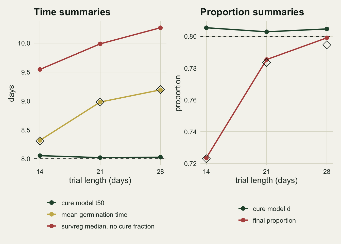
When the slow seeds have not finished, d is not there to estimate
The cure model separates speed from viability only when the trial has run long enough for the germinable seeds to show where their curve levels off. At day 14 a lot with a median of 12 days has reached F(T) = 0.649 of its germinable seeds, and nothing in the counts marks the plateau: a curve still rising at day 14 is compatible with a high d and a slow median, or with a lower d reached sooner. The chunk keeps the trial at 14 days and d at 0.8 and slows the lot down step by step.
t50_steps <- c(8, 10, 12, 14, 17, 20)
set.seed(6092)
ident <- do.call(rbind, lapply(t50_steps, function(t50_s) {
  runs <- t(replicate(n_rep, {
    fc <- fit_cure(sim_counts(n_seed, d_set, t50_s, b_set, 14), n_seed)
    c(d_hat = plogis(fc$par[1]), cov = abs(fc$par[1] - qlogis(d_set)) < 1.96 * fc$se[1])
  }))
  data.frame(t50 = t50_s, F_T = F_ll(14, t50_s, b_set), d_hat = runs[, "d_hat"], cov = runs[, "cov"])
}))
ident_sum <- do.call(rbind, lapply(split(ident, ident$t50), function(g) data.frame(
  t50 = g$t50[1], F_T = g$F_T[1], med = median(g$d_hat),
  q10 = quantile(g$d_hat, 0.1), q90 = quantile(g$d_hat, 0.9),
  at_one = mean(g$d_hat > 0.99), cov = mean(g$cov, na.rm = TRUE), cov_na = sum(is.na(g$cov)))))
round(ident_sum, 3)
t50 F_T med q10 q90 at_one cov cov_na
8 8 0.904 0.801 0.728 0.875 0.010 0.948 0
10 10 0.793 0.797 0.684 0.960 0.070 0.895 0
12 12 0.649 0.785 0.596 0.999 0.210 0.850 0
14 14 0.500 0.757 0.498 0.999 0.285 0.825 0
17 17 0.315 0.646 0.303 0.998 0.305 0.717 0
20 20 0.194 0.418 0.157 0.996 0.230 0.623 0i12 <- ident_sum[ident_sum$t50 == 12, ]; i8 <- ident_sum[ident_sum$t50 == 8, ]; i20 <- ident_sum[ident_sum$t50 == 20, ]When the lot has a median of 8 days, a 14-day trial sees 0.904 of its germinable seeds germinate, and the estimates of d are tight: the middle 80 per cent of trials lie between 0.728 and 0.875, and the Wald interval on the logit scale covers the truth in 0.948 of trials. At a median of 12 days, the slow lot of the previous section, the median estimate is still 0.785, but 0.210 of trials put d above 0.99, the upper decile is 0.999, and coverage has fallen to 0.850. The estimate has not become biased on average so much as unusable in a single trial: one trial in five says every seed is germinable and the rest are merely slow. By a median of 20 days, when only 0.194 of germinable seeds germinate within the trial, the median estimate is 0.418 and coverage 0.623.
This is the “sufficient follow-up” condition of cure models in survival analysis, as in the latency post, and it is where the answer to the 14-day comparison above has to be qualified. The likelihood ratio test for d kept its level there, but that is not the same as working. The fourth scenario of the pairs chunk puts a real difference in d, 0.8 against 0.6, on two lots that both have a median of 12 days: the cure-model test for d rejected in only 0.098 of those pairs, against 0.510 when both lots had a median of 8 days, while the final-count test still rejected in 0.428 (exact 0.416). On lots this slow the final count still carries the difference, because d F(T) differs, but it would carry a difference in speed just as readily, and the test built to tell the two apart has little power left. What a 14-day trial on a slow lot can support is a statement about germination by day 14, not a statement about viability. The fitted curve shows which case applies: if d F(T) is well below d, the plateau was not observed.
ident$lab <- factor(sprintf("t50 %d\nF(14) %.2f", ident$t50, ident$F_T),
                    levels = sprintf("t50 %d\nF(14) %.2f", t50_steps, F_ll(14, t50_steps, b_set)))
ggplot(ident, aes(lab, d_hat)) +
  geom_hline(yintercept = d_set, colour = te_ink, linetype = "dashed", linewidth = 0.5) +
  geom_jitter(width = 0.25, height = 0, size = 0.7, alpha = 0.45, colour = te_forest) +
  geom_boxplot(fill = NA, colour = te_ink, outlier.shape = NA, width = 0.5, linewidth = 0.5) +
  labs(x = "median germination time t50 of the lot, and F(14) for its germinable seeds",
       y = "estimated germinable fraction",
       title = "A 14-day trial loses the plateau of a slow lot",
       subtitle = "dashed line: true germinable fraction 0.8") +
  theme_datasheet()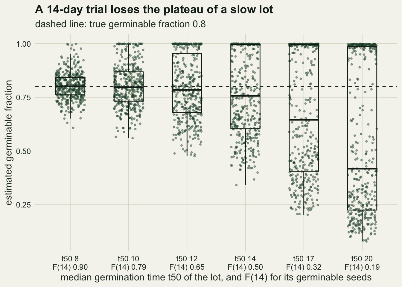
The running-total curve and its interval
A common analysis in germination papers is neither of the above. Ritz, Pipper and Streibig (2013) set the event-time fit against nonlinear regression on the running totals for germination data; the numbers below repeat that comparison by simulation. It fits a three-parameter log-logistic to the cumulative proportion germinated on each check day with nls, which returns an upper limit, a t50 and a slope, each with a standard error. The running totals are treated as independent observations with constant variance, which they are not: the total on day 10 contains the total on day 9, so the residuals are strongly positively correlated, and an extra day of checks adds a data point without adding a seed. This is the same problem Estimating R0 from incidence data shows for epidemic curves, and the numbers below come from the same trials simulated in the section on trial length.
cov_tab <- cell_sum[, c("d", "t_end", "nls_cov", "wald_cov", "prof_cov", "sr_cov",
                        "nls_se", "nls_sd", "cure_sd", "nls_w", "wald_w", "prof_w", "nls_dcov", "cure_dcov")]
round(cov_tab, 3)
d t_end nls_cov wald_cov prof_cov sr_cov nls_se nls_sd cure_sd nls_w
1 0.60 14 0.445 0.948 NaN 0.000 0.228 0.702 0.658 0.892
2 0.60 21 0.305 0.948 NaN 0.000 0.105 0.498 0.493 0.411
3 0.60 28 0.245 0.935 NaN 0.000 0.078 0.468 0.461 0.304
4 0.80 14 0.495 0.958 0.940 0.192 0.199 0.585 0.539 0.781
5 0.80 21 0.308 0.958 0.953 0.110 0.089 0.422 0.408 0.347
6 0.80 28 0.220 0.943 0.948 0.105 0.067 0.418 0.405 0.261
7 0.95 14 0.472 0.922 NaN 0.860 0.179 0.526 0.424 0.703
8 0.95 21 0.322 0.945 NaN 0.863 0.082 0.391 0.375 0.320
9 0.95 28 0.258 0.938 NaN 0.870 0.061 0.371 0.367 0.238
wald_w prof_w nls_dcov cure_dcov
1 2.467 NaN 0.448 0.953
2 1.857 NaN 0.190 0.943
3 1.795 NaN 0.102 0.955
4 2.078 2.240 0.560 0.973
5 1.597 1.642 0.265 0.958
6 1.532 1.556 0.145 0.950
7 1.697 NaN 0.590 0.890
8 1.475 NaN 0.432 0.958
9 1.415 NaN 0.288 0.970mcse_cov <- sqrt(0.95 * 0.05 / n_rep)
fails <- c(nls = sum(cell_sum$nls_fail), prof = sum(cell_sum$prof_na),
wald = sum(cell_sum$wald_na), conv = sum(cell_sum$conv_bad))
fails nls prof wald conv
0 0 0 0 c14 <- cell_sum[row_of(14, d_set), ]; c21 <- cell_sum[row_of(21, d_set), ]; c28 <- cell_sum[row_of(28, d_set), ]
se_ratio_21 <- c21$nls_sd / c21$nls_se
wald_rng <- range(cell_sum$wald_cov); nls_rng <- range(cell_sum$nls_cov)
nls_d_rng <- range(cell_sum$nls_dcov); cure_d_rng <- range(cell_sum$cure_dcov)
wald_low <- cell_sum[which.min(cell_sum$wald_cov), ]
dcov_low <- cell_sum[which.min(cell_sum$cure_dcov), ]The nls point estimates are fine: at d = 0.8 their spread across trials, 0.422 days at 21 days, is close to that of the cure model, 0.408. The standard error nls reports is not. It averaged 0.089 days, so the real spread is 4.8 times the reported one, and a 1.96-standard-error interval from the reported standard error covered the true t50 in 0.495 of 14-day trials, 0.308 of 21-day trials and 0.220 of 28-day trials. Running the trial longer makes it worse, because each extra check day adds a point to the plateau that the fit counts as new information. Across all nine cells the nls coverage for t50 ranged from 0.220 to 0.495, and for the upper limit d from 0.102 to 0.590.
The cure-model Wald interval for t50, built on the log scale, covered in between 0.922 and 0.958 of trials across the nine cells, against a Monte Carlo standard error of 0.011 at 0.95; the lowest value, in the cell with d = 0.95 and a 14-day trial, is 2.5 standard errors below the nominal level. The profile likelihood interval, computed at d = 0.8, covered 0.940, 0.953 and 0.948, with average widths of 2.24, 1.64 and 1.56 days; the Wald widths were 2.08, 1.60 and 1.53. The Wald interval for d, on the logit scale, covered between 0.890 and 0.973; the lowest, in the cell with d = 0.95 and a 14-day trial, is 5.5 standard errors low, as a logit Wald interval near the boundary tends to be. survreg without a cure fraction covered in 0.110 of 21-day trials at d = 0.8, because its interval is centred on the wrong median. Every nls fit converged, every cure-model fit reported convergence and returned an invertible Hessian, and every profile interval found both ends (failure counts 0, 0, 0 and 0).
cov_long <- data.frame(d = rep(cell_sum$d, 4), t_end = rep(cell_sum$t_end, 4),
  method = rep(c("nls on running totals", "cure model, Wald", "cure model, profile", "survreg, no cure fraction"),
               each = nrow(cell_sum)),
  coverage = c(cell_sum$nls_cov, cell_sum$wald_cov, cell_sum$prof_cov, cell_sum$sr_cov))
cov_long <- cov_long[is.finite(cov_long$coverage), ]
cov_long$d_lab <- factor(paste("germinable fraction", cov_long$d))
cov_long$method <- factor(cov_long$method, levels = c("nls on running totals", "survreg, no cure fraction",
                                                      "cure model, Wald", "cure model, profile"))
ggplot(cov_long, aes(t_end, coverage, colour = method)) +
  annotate("rect", xmin = -Inf, xmax = Inf, ymin = 0.95 - 2 * mcse_cov, ymax = 0.95 + 2 * mcse_cov,
           fill = te_line, alpha = 0.6) +
  geom_line(aes(linetype = method), linewidth = 0.9) + geom_point(size = 2.4) +
  facet_wrap(~ d_lab, nrow = 1) +
  scale_linetype_manual(values = c("solid", "solid", "solid", "22"), name = NULL) +
  scale_colour_manual(values = c(te_rust, te_gold, te_forest, te_ink), name = NULL) +
  scale_x_continuous(breaks = c(14, 21, 28)) +
  scale_y_continuous(limits = c(0, 1)) +
  labs(x = "trial length (days)", y = "coverage of the true t50",
       title = "Only the cure-model t50 intervals hold their level") +
  theme_datasheet() + theme(legend.position = "bottom") +
  guides(colour = guide_legend(nrow = 2))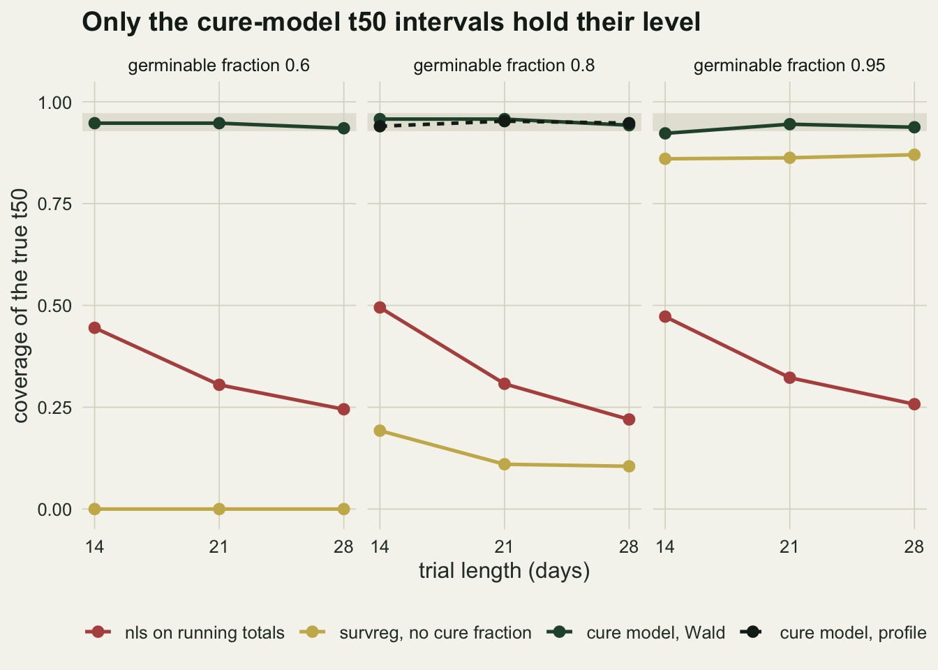
Dishes are not seeds
The trials above treat 100 seeds as independent. The nursery’s 100 seeds sat in four dishes of 25, and dishes differ: one gets a fungal infection, one dries out a little faster. The chunk gives each dish its own germinable fraction from a beta distribution with mean 0.8 and an intra-dish correlation of 0.1, a value fixed before the run, and fits the same pooled cure model to the summed counts.
rho_dish <- 0.1
n_dish <- 4; per_dish <- 25
a_beta <- d_set * (1 / rho_dish - 1); b_beta <- (1 - d_set) * (1 / rho_dish - 1)
set.seed(7730)
dish_runs <- t(replicate(n_rep, {
  d_dish <- rbeta(n_dish, a_beta, b_beta)
  cnt <- Reduce(`+`, lapply(d_dish, function(dd) sim_counts(per_dish, dd, t50_set, b_set, 21)))
  fc <- fit_cure(cnt, n_seed)
  c(d_cov = abs(fc$par[1] - qlogis(d_set)) < 1.96 * fc$se[1],
    t50_cov = abs(fc$par[2] - log(t50_set)) < 1.96 * fc$se[2])
}))
dish_cov <- colMeans(dish_runs, na.rm = TRUE)
dish_na <- sum(!is.finite(dish_runs))
var_infl <- 1 + (per_dish - 1) * rho_dish
F_21 <- F_ll(21, t50_set, b_set)
icc_germ <- F_21^2 * rho_dish * d_set * (1 - d_set) / (d_set * F_21 * (1 - d_set * F_21))
var_infl_germ <- 1 + (per_dish - 1) * icc_germ
round(c(dish_cov, na = dish_na, var_inflation = var_infl), 3)
d_cov t50_cov na var_inflation
0.738 0.950 0.000 3.400 Trials without dish variation covered the true d in 0.958 of 21-day trials. With dishes, the pooled fit’s interval for d covered in 0.738, while the interval for t50 covered in 0.950, because in this generator the dishes differ in how many seeds can germinate and not in how fast. For a plain count, the variance of a total over dishes of 25 is inflated by the design effect 1 + (25 - 1) times the intra-dish correlation: 3.4 for the germinable seeds, and 3.2 for the seeds germinated by day 21, whose intra-dish correlation is 0.090. That is the factor the pooled likelihood ignores. The four dishes, not the hundred seeds, are the replicates for d; the dish counts should be kept separate on the lab sheet so that a dish-level model, or at the least an interval whose width is multiplied by the square root of that factor, is possible. Pseudoreplication and false positives in ecology covers the general case.
What to report
Keep the counts per check day and per dish, with the check days as recorded. The final percentage, mean germination time and a fitted curve can all be rebuilt from that table; none of them can be turned back into it.
State the trial length next to every summary. A final percentage or a mean germination time without the day the trial stopped is not comparable with a study that stopped on another day; seed-testing rules fix the final count day for crop species for this reason, but most wild-species trials have no such rule, and in the simulations above the same seeds moved both summaries with trial length alone.
Fit the interval-censored likelihood with a germinable fraction and report d and t50 separately, each with an interval; the profile interval for t50 costs one uniroot per end. Test a treatment effect on d and on t50 separately. On a trial that stopped before the plateau, a non-significant test on d is not evidence of equal viability. If only a final-count test is reported, say that it cannot separate speed from viability.
Check the plateau before interpreting d. If the fitted d F(T) is well short of d, or the running total is still rising on the last check days, the trial did not run long enough to estimate a germinable fraction, and d should be reported as not identified rather than as a number near one.
If the ungerminated seeds were tested with tetrazolium at the end of the trial, report that count as well. It is a check on the model, not a replacement for it. The seeds the cure model calls non-germinable include dormant live seeds, which tetrazolium stains as viable, so 1 - d should be at least the tetrazolium dead fraction; if it is much smaller, d has probably been overestimated, which is the pattern of a trial stopped before the plateau.
Do not report the nls standard errors of a curve fitted to running totals. If a cumulative curve is the familiar picture for readers, draw it from the event-time fit.
Honest limits
Every trial here was generated by a log-logistic germination curve with a single germinable fraction, and every model fitted that same curve. Real lots mix seeds with different dormancy, which gives two waves of germination or a long shallow tail. A cure model with one log-logistic would then fit a compromise, and the germinable fraction would absorb part of the slow wave; nothing above measures how badly.
The checks are daily and none is missed. Labs that skip weekends have wider intervals on some days, which the interval likelihood handles directly, while nls and mean germination time silently assign the germinations to the next check day. That case was not simulated.
The dish section varies only the germinable fraction between dishes. Dishes that also differ in speed, through moisture or temperature position in the cabinet, would push the t50 interval below its level too. The repairs, a dish-level random effect in the likelihood or a bootstrap over dishes, were not simulated, and with four dishes per lot neither has much to work with.
The speed-only comparison used 100 seeds per lot, a median of 8 against 12 days and one slope. With more seeds the final-count test rejects more often, not less, because the confusion is a real difference in d F(T) and a bigger sample detects it better; the exact rejection function in the post can be rerun for another design in a second.
Temperature and water potential enter germination through thermal-time and hydrotime models, which move t50 with the environment. The cure model here is the building block those models extend, and nothing here tests them. Coverage and rejection rates are estimated from 400 simulated trials or pairs, so one Monte Carlo standard error for a rate is 0.011 at a rate of 0.05 and 0.025, its largest, at 0.5, and a single rate can land two standard errors away, as the simulated final-count rate at 14 days did (0.850 against an exact 0.811).
References
Farewell VT 1982 Biometrics 38(4):1041-1046 (10.2307/2529885)
McNair JN, Sunkara A, Frobish D 2012 Seed Science Research 22(2):77-95 (10.1017/S0960258511000547)
Onofri A, Gresta F, Tei F 2010 Weed Research 50(3):187-198 (10.1111/j.1365-3180.2010.00776.x)
Onofri A, Mesgaran MB, Tei F, Cousens RD 2011 Weed Research 51(5):516-524 (10.1111/j.1365-3180.2011.00870.x)
Ritz C, Pipper CB, Streibig JC 2013 European Journal of Agronomy 45:1-6 (10.1016/j.eja.2012.10.003)