library(ggplot2)
library(patchwork)
library(survival)

te_paper  <- "#f5f4ee"
te_ink    <- "#16241d"
te_body   <- "#2c3a31"
te_forest <- "#275139"
te_rust   <- "#b5534e"
te_gold   <- "#c9b458"
te_line   <- "#dad9ca"

theme_datasheet <- function() {
  theme_minimal(base_size = 12) +
    theme(plot.background  = element_rect(fill = te_paper, colour = NA),
          panel.background = element_rect(fill = te_paper, colour = NA),
          panel.grid.major = element_line(colour = te_line, linewidth = 0.3),
          panel.grid.minor = element_blank(),
          text             = element_text(colour = te_body),
          plot.title       = element_text(colour = te_ink, face = "bold"),
          plot.subtitle    = element_text(colour = te_body),
          axis.text        = element_text(colour = te_body),
          strip.text       = element_text(colour = te_ink))
}Latency tests when some animals never respond
R
survival analysis
animal behaviour
simulation
ecology tutorial
Novel-object latency tests with non-responders mix two effects. Measuring in R how Cox, t tests and a mixture cure model read more responders or faster ones.
A novel object goes into the aviary next to the feeder, and a camera records how long each great tit takes to land on the feeder again. The trial stops at 300 seconds. Some birds come back within a minute, some take four, and a good share never come back while the camera runs. The experiment compares two groups: birds raised with extra environmental enrichment and control birds. The spreadsheet has one latency per bird, with 300 written in for the birds that did not return.
Two routine analyses follow. One takes the log of the recorded latency, 300 included, and runs a t test. The other, recommended by Jahn-Eimermacher and colleagues for latency outcomes because an ANOVA “cannot properly deal with animals not showing the performance measure within the trial time”, treats the birds that did not return as censored at 300 and applies survival analysis, typically a log-rank test or a Cox model. The second is the better habit. It still assumes something the data may not support: that a bird censored at 300 seconds would have returned at some later time.
For many behavioural latencies that is not true. A bird that is strongly neophobic, or not hungry that morning, would not approach in ten minutes or in an hour. The population has two kinds of individual: responders, with a latency distribution, and non-responders, with no latency at all. A treatment can change the share of responders, the speed of the responders, or both, and these are different biological effects. Berkson and Gage wrote down the survival model for this situation in 1952, for cancer patients some of whom are cured, and Farewell gave it the form used here: a logistic regression for whether the event ever happens and a parametric survival model for when it happens among those for whom it does. This post is a demonstration of that model on a latency test, and what it measures is how the everyday tests read each kind of treatment effect.
The four survival posts this one builds on assume that every animal eventually has the event. Kaplan-Meier survival curves and the log-rank test shows why the naive mean of censored times misleads, with lifespans that end in death for every animal. Cox proportional hazards and the PH assumption handles hazards that cross because juveniles and adults die at different ages, not a plateau. Checking a survival model measures the low power of the proportional hazards test and how an omitted covariate fakes a violation, and Parametric survival and the AFT model shows how the tail beyond the data belongs to the chosen distribution. Here the curve flattens out above zero because part of the sample never responds, and that plateau folds two treatment effects into one hazard ratio. A cumulative curve that stops short of one is not new on the site: in Competing risks and cumulative incidence an animal killed by another cause can never have the event of interest, but there every animal still has some event, whereas here the non-responder has none. Germination trials as time-to-event data fits the same cure fraction to seed lots, where the question is viability against speed; this post asks the same question of a behavioural latency with right censoring at a fixed cap.
A plateau under the curve
Each simulated experiment has 30 birds per group and a 300 s cap. A bird is a responder with probability p, and a responder’s latency is exponential with mean m seconds. Four scenarios were fixed before any run. With no effect, both groups have p = 0.6 and m = 60. With more responders, the treated group has p = 0.8 against 0.5 and the same speed. With faster responders, both groups have p = 0.6 and the treated responders have a mean latency of 30 s against 60. With faster but fewer, the treated group has p = 0.5 and m = 20 against a control of p = 0.8 and m = 60: enrichment makes some birds bolder and quicker while others stop approaching at all.
The cure model has four parameters: the log odds of responding in the control group, the log rate of responding among control responders, and a treatment effect on each. An animal that responds at time y contributes p times the exponential density at y; an animal still waiting at the cap contributes 1 - p + p exp(-rate x 300), the chance that it is a non-responder or a responder that has not yet come. Each effect is tested with a likelihood ratio test against the model with that effect set to zero. The code fits the model with optim() and an analytic gradient, and refits the full model if a restricted fit ever comes out better, which would mean the first fit stopped early.
trial_cap <- 300
n_group   <- 30

scenarios <- data.frame(
  scenario = c("no effect", "more responders", "faster responders",
               "faster but fewer"),
  p_control = c(0.6, 0.5, 0.6, 0.8), p_treated = c(0.6, 0.8, 0.6, 0.5),
  m_control = c(60, 60, 60, 60),     m_treated = c(60, 60, 30, 20))

simulate_trial <- function(n, p_c, p_t, m_c, m_t, shape = 1, cap = trial_cap) {
  group <- rep(0:1, each = n)
  p_resp <- ifelse(group == 1, p_t, p_c)
  mean_lat <- ifelse(group == 1, m_t, m_c)
  scale_w <- mean_lat / gamma(1 + 1 / shape)
  latency <- ifelse(runif(2 * n) < p_resp, rweibull(2 * n, shape, scale_w), Inf)
  data.frame(group = group, time = pmin(latency, cap),
             status = as.numeric(latency <= cap))
}

# Exponential mixture cure model: logit share of responders, log rate among
# responders; par = (a0, b0, a1, b1), a1 and b1 are the treatment effects
cure_nll <- function(par, time, status, group) {
  p_r <- plogis(par[1] + par[3] * group)
  rate <- exp(par[2] + par[4] * group)
  surv_r <- exp(-rate * time)
  -sum(status * (log(p_r) + log(rate) - rate * time) +
         (1 - status) * log(1 - p_r + p_r * surv_r))
}
cure_grad <- function(par, time, status, group) {
  p_r <- plogis(par[1] + par[3] * group)
  rate <- exp(par[2] + par[4] * group)
  surv_r <- exp(-rate * time)
  lik_c <- 1 - p_r + p_r * surv_r
  g_a <- status * (1 - p_r) + (1 - status) * p_r * (1 - p_r) * (surv_r - 1) / lik_c
  g_b <- status * (1 - rate * time) - (1 - status) * p_r * surv_r * rate * time / lik_c
  -c(sum(g_a), sum(g_b), sum(g_a * group), sum(g_b * group))
}

# Weibull version: one shared shape, par[5] = log shape
cure_nll_weib <- function(par, time, status, group) {
  p_r <- plogis(par[1] + par[3] * group)
  rate <- exp(par[2] + par[4] * group)
  shape <- exp(par[5])
  cum_h <- (rate * time)^shape
  -sum(status * (log(p_r) + log(shape) + shape * log(rate) +
                   (shape - 1) * log(time) - cum_h) +
         (1 - status) * log(1 - p_r + p_r * exp(-cum_h)))
}

fit_one <- function(dat, fix, start_par, weibull) {
  n_par <- if (weibull) 5 else 4
  free <- setdiff(seq_len(n_par), fix)
  full_par <- function(q) { par <- rep(0, n_par); par[free] <- q; par }
  fn <- function(q) {
    if (weibull) cure_nll_weib(full_par(q), dat$time, dat$status, dat$group)
    else cure_nll(full_par(q), dat$time, dat$status, dat$group)
  }
  gr <- if (weibull) NULL else function(q) {
    cure_grad(full_par(q), dat$time, dat$status, dat$group)[free]
  }
  opt <- optim(start_par[free], fn, gr, method = "BFGS", control = list(maxit = 500))
  list(value = opt$value, par = full_par(opt$par), fn = fn, gr = gr, free = free,
       conv = opt$convergence)
}

# Full fit and the two restricted fits (no incidence effect, no speed effect).
# A restricted fit that beats the full fit means the full fit stopped early:
# refit the full model from there.
cure_tests <- function(dat, weibull = FALSE, hessian = FALSE) {
  resp <- dat$status == 1
  start_par <- c(qlogis(min(max(mean(resp), 0.05), 0.95)),
             log(sum(resp) / sum(dat$time[resp])), 0, 0)
  if (weibull) start_par <- c(start_par, 0)
  full <- fit_one(dat, integer(0), start_par, weibull)
  no_inc <- fit_one(dat, 3, full$par, weibull)
  no_spd <- fit_one(dat, 4, full$par, weibull)
  best <- which.min(c(full$value, no_inc$value, no_spd$value))
  if (best > 1) {
    full <- fit_one(dat, integer(0), list(full, no_inc, no_spd)[[best]]$par, weibull)
  }
  out <- c(lrt_inc = 2 * (no_inc$value - full$value),
           lrt_spd = 2 * (no_spd$value - full$value),
           a0 = full$par[1], b0 = full$par[2], a1 = full$par[3], b1 = full$par[4],
           conv = full$conv + no_inc$conv + no_spd$conv)
  if (hessian) {
    hess <- optimHess(full$par, full$fn, full$gr)
    vc <- tryCatch(solve(hess), error = function(e) matrix(NA, 4, 4))
    safe_se <- function(v) if (is.na(v) || v <= 0) NA_real_ else sqrt(v)
    out <- c(out, se_a0 = safe_se(vc[1, 1]),
             se_at = safe_se(vc[1, 1] + vc[3, 3] + 2 * vc[1, 3]),
             se_b1 = safe_se(vc[4, 4]))
  }
  out
}
Before any simulation, the expected curves already show the problem. The hazard for the whole group at time t is p rate exp(-rate t) / (1 - p + p exp(-rate t)). It falls over the trial even though each responder’s hazard is constant, because the animals still waiting are more and more likely to be non-responders.
hazard_ratio_true <- function(t, p_c, p_t, m_c, m_t) {
  haz <- function(p, m) p * exp(-t / m) / m / (1 - p + p * exp(-t / m))
  haz(p_t, m_t) / haz(p_c, m_c)
}
curve_grid <- seq(0, trial_cap, by = 1)
curve_df <- do.call(rbind, lapply(2:4, function(i) {
  s <- scenarios[i, ]
  rbind(data.frame(scenario = s$scenario, time = curve_grid, group = "control",
                   still_waiting = 1 - s$p_control * (1 - exp(-curve_grid / s$m_control))),
        data.frame(scenario = s$scenario, time = curve_grid, group = "treated",
                   still_waiting = 1 - s$p_treated * (1 - exp(-curve_grid / s$m_treated))))
}))
hr_df <- do.call(rbind, lapply(2:4, function(i) {
  s <- scenarios[i, ]
  data.frame(scenario = s$scenario, time = curve_grid,
             hr = hazard_ratio_true(curve_grid, s$p_control, s$p_treated,
                                    s$m_control, s$m_treated))
}))
hr_at <- function(scen, t) hr_df$hr[hr_df$scenario == scen & hr_df$time == t]
odds_ratio_more <- (0.8 / 0.2) / (0.5 / 0.5)
With more responders and equal speed, the ratio of treated to control hazard starts at the ratio of the response shares, 1.6, and climbs towards the ratio of the odds of responding, 4; at the cap it is 3.92. The hazards are not proportional, but the ratio stays above one and changes slowly. With faster responders and equal shares, the ratio starts at 2 and falls to 0.014 at the cap, because by then the treated birds that were going to come have come. A single hazard ratio averages over these curves with weights set by when the events happen.
lev <- scenarios$scenario[2:4]
curve_df$scenario <- factor(curve_df$scenario, levels = lev)
hr_df$scenario <- factor(hr_df$scenario, levels = lev)
p_surv <- ggplot(curve_df, aes(time, still_waiting, colour = group)) +
  geom_line(linewidth = 0.9) +
  facet_wrap(~ scenario) +
  scale_colour_manual(values = c(control = te_ink, treated = te_rust), name = NULL) +
  scale_y_continuous(limits = c(0, 1)) +
  scale_x_continuous(breaks = c(0, 100, 200, 300)) +
  labs(x = NULL, y = "share not yet responded",
       title = "Three treatments, three shapes of plateau",
       subtitle = "expected curves; responders' latency exponential; 300 s cap") +
  theme_datasheet() +
  theme(legend.position = "top")
p_hr <- ggplot(hr_df, aes(time, hr)) +
  geom_hline(yintercept = 1, linetype = "dashed", colour = te_body, linewidth = 0.4) +
  geom_line(colour = te_forest, linewidth = 0.9) +
  facet_wrap(~ scenario) +
  scale_y_log10(breaks = c(0.01, 0.1, 1, 10), labels = c("0.01", "0.1", "1", "10")) +
  coord_cartesian(ylim = c(0.01, 10)) +
  scale_x_continuous(breaks = c(0, 100, 200, 300)) +
  labs(x = "seconds since the object was placed", y = "true hazard ratio",
       subtitle = "treated / control hazard, log scale") +
  theme_datasheet()
(p_surv / p_hr) + plot_annotation(theme = theme_datasheet())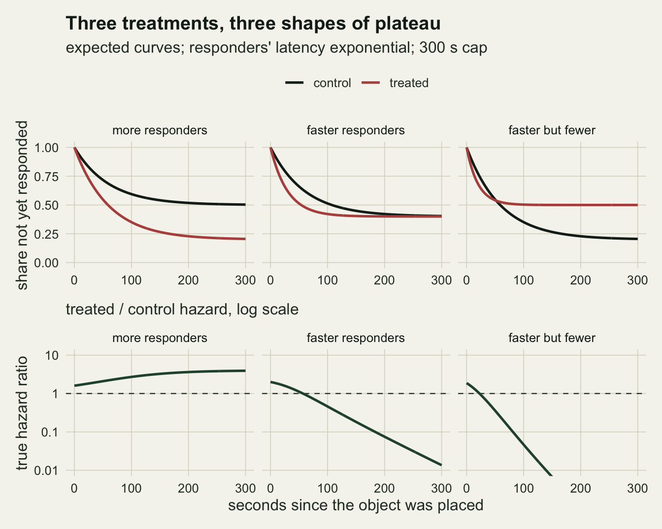
What each test reports
Each of the four scenarios gets 1000 simulated experiments. Every experiment is analysed eight ways: a t test on log latency with the non-responders entered at 300 s, a t test on log latency of the responders only, a Mann-Whitney test on the capped latency, the log-rank test, the Wald test of a Cox model, the proportional hazards test from cox.zph(), and the two likelihood ratio tests of the cure model. The Cox hazard ratio is treated over control, so a value above one means the treated birds return sooner.
n_rep <- 1000
one_experiment <- function(s) {
  dat <- simulate_trial(n_group, s$p_control, s$p_treated, s$m_control, s$m_treated)
  cox_fit <- coxph(Surv(time, status) ~ group, data = dat)
  resp <- dat[dat$status == 1, ]
  p_drop <- if (min(table(factor(resp$group, 0:1))) >= 2) {
    t.test(log(time) ~ group, data = resp)$p.value
  } else NA
  cure <- cure_tests(dat, hessian = TRUE)
  c(t_capped = t.test(log(time) ~ group, data = dat)$p.value,
    t_responders = p_drop,
    mann_whitney = wilcox.test(time ~ group, data = dat, exact = FALSE)$p.value,
    log_rank = pchisq(survdiff(Surv(time, status) ~ group, data = dat)$chisq, 1,
                      lower.tail = FALSE),
    cox = summary(cox_fit)$coefficients[1, 5],
    ph_test = cox.zph(cox_fit)$table[1, 3],
    cure_inc = pchisq(cure[["lrt_inc"]], 1, lower.tail = FALSE),
    cure_spd = pchisq(cure[["lrt_spd"]], 1, lower.tail = FALSE),
    hr = exp(coef(cox_fit)[[1]]), cure)
}

set.seed(1952)
sim_main <- lapply(seq_len(nrow(scenarios)), function(i) {
  t(replicate(n_rep, one_experiment(scenarios[i, ])))
})
names(sim_main) <- scenarios$scenario

test_cols <- c("t_capped", "t_responders", "mann_whitney", "log_rank", "cox",
               "ph_test", "cure_inc", "cure_spd")
test_labels <- c("t test, capped log latency", "t test, responders only",
                 "Mann-Whitney, capped latency", "log-rank", "Cox",
                 "PH test (cox.zph)", "cure model: incidence LRT",
                 "cure model: speed LRT")
rej_tab <- do.call(rbind, lapply(names(sim_main), function(sc) {
  m <- sim_main[[sc]]
  data.frame(scenario = sc, test = test_labels,
             rate = colMeans(m[, test_cols] < 0.05, na.rm = TRUE),
             n_used = colSums(!is.na(m[, test_cols])))
}))
rej <- function(sc, col) mean(sim_main[[sc]][, col] < 0.05, na.rm = TRUE)
med_hr <- function(sc) median(sim_main[[sc]][, "hr"])
share_hr_up <- function(sc) mean(sim_main[[sc]][, "hr"] > 1)
mc_se_05 <- sqrt(0.05 * 0.95 / n_rep)
mc_se_max <- sqrt(0.25 / n_rep)
n_drop_na <- sum(is.na(unlist(lapply(sim_main, function(m) m[, "t_responders"]))))
n_nonconv <- sum(unlist(lapply(sim_main, function(m) m[, "conv"])) > 0)

coverage_of <- function(sc) {
  m <- sim_main[[sc]]; s <- scenarios[scenarios$scenario == sc, ]
  a_true <- qlogis(s$p_control); at_true <- qlogis(s$p_treated)
  b1_true <- log(s$m_control / s$m_treated)
  cover <- function(est, se, truth) mean(!is.na(se) & abs(est - truth) <= 1.96 * se)
  c(p_control = cover(m[, "a0"], m[, "se_a0"], a_true),
    p_treated = cover(m[, "a0"] + m[, "a1"], m[, "se_at"], at_true),
    rate_ratio = cover(m[, "b1"], m[, "se_b1"], b1_true),
    bias_pc = median(plogis(m[, "a0"])) - s$p_control,
    bias_pt = median(plogis(m[, "a0"] + m[, "a1"])) - s$p_treated,
    rr_med = median(exp(m[, "b1"])), rr_true = exp(b1_true))
}
cov_tab <- sapply(scenarios$scenario, coverage_of)
The Monte Carlo standard error of a rejection rate near 0.05 is 0.0069 with 1000 experiments, and at most 0.016 for any rate. With no effect every test rejects in 0.035 to 0.057 of experiments; the lowest is the t test on responders only. The responders-only test needs two responders in each group; the number of experiments that failed this was 0, and the number with a cure-model fit reporting non-convergence was 0.
More responders. The Cox model reports a median hazard ratio of 2.20, above one in 0.990 of experiments, and rejects in 0.647. Read in the usual way, enriched birds return about twice as fast. They do not: responders in both groups have the same mean latency, and the t test on responders only rejects in 0.048. The proportional hazards test flags the model in only 0.127 of experiments, because over the first two minutes, when most birds that return do so, the true hazard ratio only drifts in one direction from 1.6 to 2.9, a trend too gentle for the test to see in samples of this size. The cure model’s incidence test rejects in 0.656, about the power of the Cox model, and its speed test in 0.066.
Faster responders. Here the one-number tests are weak. Cox rejects in 0.088 with a median hazard ratio of 1.18, and the log-rank test in 0.092, because the treatment changes when the responders come and not how many come, and the hazard ratio runs from above one early to far below one late. The proportional hazards test flags 0.350 of experiments. The speed test of the cure model rejects in 0.542 and the incidence test in 0.061.
Faster but fewer. The median Cox hazard ratio is 0.62, above one in only 0.074 of experiments: the model says treated birds return more slowly, and it rejects in 0.304. The t test on capped log latency rejects in 0.067 and the Mann-Whitney test in 0.107; the two effects cancel on the capped scale. Unlike the more-responders case, the proportional hazards test does flag this one, in 0.893 of experiments, so the blind spot above belongs to a pure incidence effect and not to every mixture. The cure model finds both parts: incidence in 0.694 and speed in 0.897.
The cure model also gets the numbers right, not only the tests. Across the four scenarios, its Wald intervals (on the logit scale for the shares, on the log scale for the rate ratio) cover the true control share in 0.960 to 0.972 of experiments, the treated share in 0.953 to 0.964, and the rate ratio in 0.938 to 0.962. The median estimated shares are within 0.005 of the truth, and the median rate ratio in the faster-but-fewer case is 3.10 against a true 3.
rej_plot <- rej_tab
rej_plot$test <- factor(rej_plot$test, levels = rev(test_labels))
rej_plot$scenario <- factor(rej_plot$scenario, levels = scenarios$scenario)
rej_plot$kind <- ifelse(grepl("cure", rej_plot$test), "cure model",
                        ifelse(grepl("PH test", rej_plot$test), "assumption check",
                               "one-number test"))
ggplot(rej_plot, aes(rate, test, colour = kind, shape = kind)) +
  geom_vline(xintercept = 0.05, linetype = "dashed", colour = te_body, linewidth = 0.4) +
  geom_point(size = 2.8) +
  facet_wrap(~ scenario, nrow = 2) +
  scale_colour_manual(values = c("one-number test" = te_ink, "assumption check" = te_gold,
                                 "cure model" = te_rust), name = NULL) +
  scale_shape_manual(values = c("one-number test" = 16, "assumption check" = 17,
                                "cure model" = 15), name = NULL) +
  scale_x_continuous(limits = c(0, 1), breaks = c(0, 0.25, 0.5, 0.75, 1),
                     labels = c("0", "0.25", "0.5", "0.75", "1")) +
  labs(x = "share of experiments with p < 0.05", y = NULL,
       title = "One hazard ratio, two effects",
       subtitle = "30 animals per group, 300 s cap, 1000 experiments per panel") +
  theme_datasheet() +
  theme(legend.position = "bottom")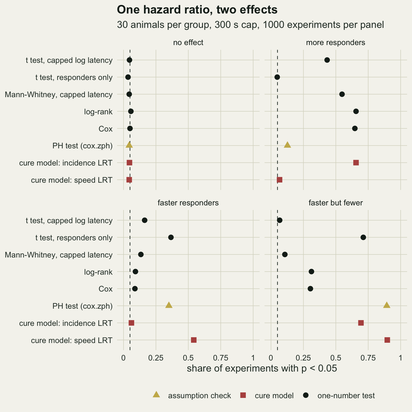
The speed test when only incidence differs
One worry about the cure model is that a difference in incidence could leak into the speed test. With few responders in one group the rate among responders is estimated from few events, and the two parameters trade off: a higher share of slow responders and a lower share of fast ones can describe a similar curve. If that trade-off mattered at these sample sizes, a pure incidence effect would push the speed test above its nominal level. The check below fits only the cure model, with equal speeds, at four group sizes and three pairs of response shares, 1000 experiments per cell.
n_leak <- 1000
leak_grid <- expand.grid(n = c(20, 30, 60, 120),
                         pair = c("0.5 and 0.5", "0.5 and 0.8", "0.8 and 0.8"),
                         stringsAsFactors = FALSE)
pair_p <- list("0.5 and 0.5" = c(0.5, 0.5), "0.5 and 0.8" = c(0.5, 0.8),
               "0.8 and 0.8" = c(0.8, 0.8))
set.seed(1982)
leak_raw <- lapply(seq_len(nrow(leak_grid)), function(i) {
  pp <- pair_p[[leak_grid$pair[i]]]
  t(replicate(n_leak, cure_tests(simulate_trial(leak_grid$n[i], pp[1], pp[2], 60, 60))
              [c("lrt_inc", "lrt_spd", "conv")]))
})
leak_grid$spd_rate <- sapply(leak_raw, function(m) mean(m[, "lrt_spd"] > qchisq(0.95, 1)))
leak_grid$spd_mean <- sapply(leak_raw, function(m) mean(m[, "lrt_spd"]))
leak_grid$inc_rate <- sapply(leak_raw, function(m) mean(m[, "lrt_inc"] > qchisq(0.95, 1)))
pooled_by <- function(col, value) {
  idx <- which(leak_grid[[col]] == value)
  all_stat <- unlist(lapply(leak_raw[idx], function(m) m[, "lrt_spd"]))
  c(rate = mean(all_stat > qchisq(0.95, 1)), n = length(all_stat),
    mean_stat = mean(all_stat))
}
leak_pair <- sapply(names(pair_p), function(v) pooled_by("pair", v))
leak_n <- sapply(c(20, 30, 60, 120), function(v) pooled_by("n", v))
leak_all <- unlist(lapply(leak_raw, function(m) m[, "lrt_spd"]))
leak_rate_all <- mean(leak_all > qchisq(0.95, 1))
leak_se_all <- sqrt(leak_rate_all * (1 - leak_rate_all) / length(leak_all))
leak_mean_all <- mean(leak_all)
leak_mean_se <- sd(leak_all) / sqrt(length(leak_all))
leak_nonconv <- sum(unlist(lapply(leak_raw, function(m) m[, "conv"])) > 0)
inc_power <- function(n) leak_grid$inc_rate[leak_grid$n == n & leak_grid$pair == "0.5 and 0.8"]
Pooled over group sizes, the speed test rejects in 0.0545 of 4000 experiments when the shares are 0.5 and 0.8, against 0.0493 when both are 0.5 and 0.0532 when both are 0.8. The Monte Carlo standard error of each pooled rate is about 0.0034. Pooled over the shares, the rate is 0.0520 at 20 birds per group and 0.0513 at 120. Over all 12000 experiments it is 0.0523 (standard error 0.0020), and the mean likelihood ratio statistic is 1.019 against 1 for a chi-squared variable with one degree of freedom. The incidence difference moves the speed test by 0.0052, and the standard error of that difference is 0.0050. At these designs, with nearly every responder coming before the cap, there is no leak worth the name; the chi-squared reference is at most slightly liberal. Meanwhile the incidence test’s power grows from 0.435 at 20 birds per group to 0.932 at 60 and 0.995 at 120.
The speed test does go wrong in two other situations, which the next two sections measure: when the latency distribution is not the one the model assumes, and when the cap comes before the responders are done.
When latency is not exponential
Real latencies are rarely exponential. A few birds come back almost at once and some responders take much longer than the rest, which is a Weibull shape below one; a habituation process with a delay gives a shape above one. The cells below keep 30 birds per group and change the true Weibull shape of the responders’ latency, holding the mean. Each experiment is fitted twice: with the exponential cure model and with a Weibull cure model that adds one shape parameter shared by both groups, as in Farewell’s form. There are 600 experiments per cell.
n_shape <- 600
shape_cells <- data.frame(
  cell = c("no effect, shape 0.5", "no effect, shape 1", "no effect, shape 1.5",
           "more responders, shape 0.5", "faster responders, shape 0.5"),
  p_c = c(0.6, 0.6, 0.6, 0.5, 0.6), p_t = c(0.6, 0.6, 0.6, 0.8, 0.6),
  m_c = 60, m_t = c(60, 60, 60, 60, 30), shape = c(0.5, 1, 1.5, 0.5, 0.5))
set.seed(2000)
shape_raw <- lapply(seq_len(nrow(shape_cells)), function(i) {
  s <- shape_cells[i, ]
  t(replicate(n_shape, {
    dat <- simulate_trial(n_group, s$p_c, s$p_t, s$m_c, s$m_t, s$shape)
    e_fit <- cure_tests(dat)
    w_fit <- cure_tests(dat, weibull = TRUE)
    c(e_inc = e_fit[["lrt_inc"]], e_spd = e_fit[["lrt_spd"]],
      w_inc = w_fit[["lrt_inc"]], w_spd = w_fit[["lrt_spd"]],
      conv = e_fit[["conv"]] + w_fit[["conv"]])
  }))
})
crit <- qchisq(0.95, 1)
shape_tab <- do.call(rbind, lapply(seq_len(nrow(shape_cells)), function(i) {
  m <- shape_raw[[i]]
  data.frame(cell = shape_cells$cell[i],
             model = rep(c("exponential latency", "Weibull latency"), each = 2),
             test = rep(c("incidence LRT", "speed LRT"), 2),
             rate = c(mean(m[, "e_inc"] > crit), mean(m[, "e_spd"] > crit),
                      mean(m[, "w_inc"] > crit), mean(m[, "w_spd"] > crit)))
}))
sh <- function(cell, model, test) {
  shape_tab$rate[shape_tab$cell == cell & shape_tab$model == model & shape_tab$test == test]
}
shape_nonconv <- sum(unlist(lapply(shape_raw, function(m) m[, "conv"])) > 0)
mc_se_shape <- sqrt(0.05 * 0.95 / n_shape)
reached_shape05 <- 1 - exp(-(trial_cap / (60 / gamma(3)))^0.5)
The Monte Carlo standard error of a rate near 0.05 is 0.0089. With no treatment effect at all and a true shape of 0.5, the exponential model’s speed test rejects in 0.225 of experiments. The mixture of quick and slow responders is more spread out than any exponential, and the likelihood ratio test treats that extra spread as information about a difference between groups, much as a Poisson model reads overdispersed counts. With a true shape of 1.5 the error goes the other way and the test rejects in only 0.012. The incidence test holds its level under both shapes, 0.060 and 0.047, but when only incidence differs under shape 0.5, the exponential speed test still rejects in 0.228: a false speed effect reported next to a true incidence effect.
The Weibull cure model brings the speed test back towards its level, 0.073 at shape 0.5 and 0.085 at shape 1.5. Both are above 0.05 by more than two Monte Carlo standard errors, so with 30 birds per group and one extra parameter the chi-squared reference is liberal; a parametric bootstrap of the statistic would be the next step for a real analysis. The shape costs power where the latency is widely spread: under shape 0.5 the incidence test finds the true incidence effect in 0.378 of experiments against 0.645 for the exponential model, because a long responder tail looks partly like a plateau; at this shape only 0.958 of responders arrive before the cap, close to the follow-up cliff measured in the next section. The speed test pays more: for a true halving of mean latency the Weibull model rejects in 0.123, against 0.073 with no effect, where the exponential model at shape 1 found the same halving in 0.542 of experiments; so at 30 birds per group and a widely spread latency the speed half of the model is nearly uninformative, and part of that small margin is the liberal reference itself. The exponential model’s speed rate for the true speed effect, 0.380, is not power: a test that rejects in 0.225 of null experiments has no honest power to compare. The number of experiments with a fit reporting non-convergence was 0.
shape_plot <- shape_tab
shape_plot$cell <- factor(shape_plot$cell, levels = rev(shape_cells$cell))
ggplot(shape_plot, aes(rate, cell, colour = model, shape = model)) +
  geom_vline(xintercept = 0.05, linetype = "dashed", colour = te_body, linewidth = 0.4) +
  geom_point(size = 3, position = position_dodge(width = 0.5)) +
  facet_wrap(~ test) +
  scale_colour_manual(values = c("exponential latency" = te_rust,
                                 "Weibull latency" = te_forest), name = "cure model with") +
  scale_shape_manual(values = c("exponential latency" = 16, "Weibull latency" = 17),
                     name = "cure model with") +
  scale_x_continuous(limits = c(0, 1), breaks = c(0, 0.25, 0.5, 0.75)) +
  labs(x = "share of experiments with p < 0.05", y = NULL,
       title = "A wrong latency shape miscalibrates the speed test",
       subtitle = "30 animals per group; true Weibull shape in the row label") +
  theme_datasheet() +
  theme(legend.position = "bottom")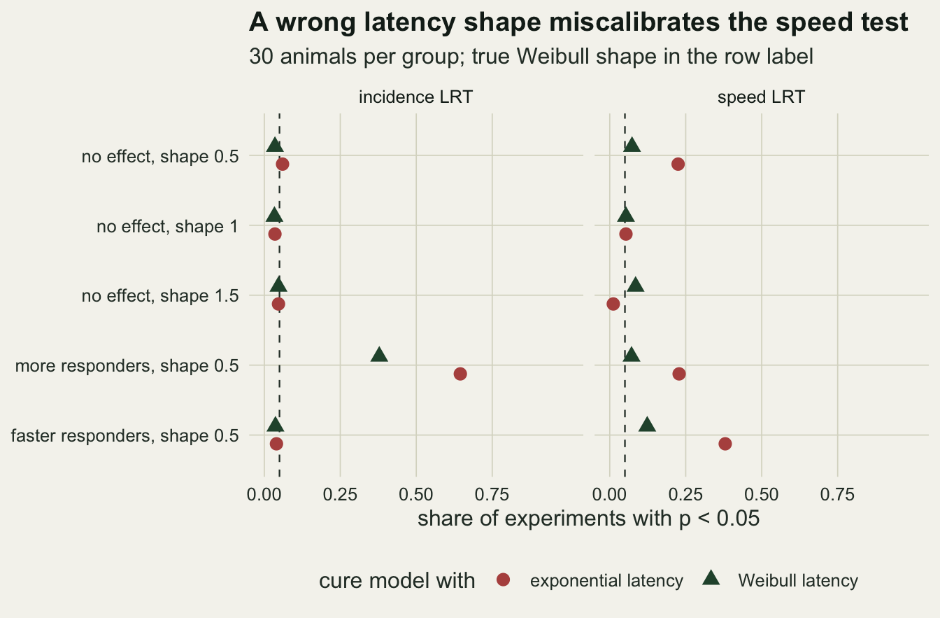
When the cap cuts into the responders
The cure model can separate a non-responder from a slow responder only if the trial lasts long enough for nearly all responders to respond. Survival statisticians call this sufficient follow-up. In the scenarios above the mean latency is 60 s and the cap is 300 s, so a responder comes before the cap with probability 0.993. The cells below keep the more-responders scenario (0.5 against 0.8) and lengthen the mean latency of both groups from 30 to 300 s under the same cap, 800 experiments per cell.
n_follow <- 800
follow_means <- c(30, 60, 100, 150, 200, 300)
set.seed(2011)
follow_raw <- lapply(follow_means, function(m) {
  t(replicate(n_follow, cure_tests(simulate_trial(n_group, 0.5, 0.8, m, m),
                                   hessian = TRUE)))
})
follow_tab <- data.frame(
  mean_latency = follow_means,
  reached = 1 - exp(-trial_cap / follow_means),
  inc_power = sapply(follow_raw, function(m) mean(m[, "lrt_inc"] > crit)),
  spd_false = sapply(follow_raw, function(m) mean(m[, "lrt_spd"] > crit)),
  cover_pc = sapply(follow_raw, function(m) {
    mean(!is.na(m[, "se_a0"]) & abs(m[, "a0"] - qlogis(0.5)) <= 1.96 * m[, "se_a0"])
  }),
  med_pc = sapply(follow_raw, function(m) median(plogis(m[, "a0"]))),
  q90_pc = sapply(follow_raw, function(m) quantile(plogis(m[, "a0"]), 0.9, names = FALSE)),
  se_na = sapply(follow_raw, function(m) mean(is.na(m[, "se_a0"]))),
  wid_pc = sapply(follow_raw, function(m) {
    se <- ifelse(is.na(m[, "se_a0"]), Inf, m[, "se_a0"])
    median(plogis(m[, "a0"] + 1.96 * se) - plogis(m[, "a0"] - 1.96 * se))
  }))
fo <- function(m, col) follow_tab[follow_tab$mean_latency == m, col]
follow_nonconv <- sum(unlist(lapply(follow_raw, function(m) m[, "conv"])) > 0)
mc_se_follow <- sqrt(0.05 * 0.95 / n_follow)
The incidence test finds the real difference in 0.704 of experiments when the mean latency is 30 s and 0.336 at 100 s, where 0.950 of responders come before the cap. At 150 s it falls to 0.156, and at 300 s, where only 0.632 of responders come in time, it rejects in 0.035, below the nominal level. The data no longer say whether a bird still waiting is a non-responder or a slow responder, so the model cannot tell a higher share from a faster rate, and the share estimates run to the boundary: at 300 s the 90th percentile of the estimated control share is 0.998, against a true 0.5.
The Wald interval for the control share still covers the truth in 0.975 of experiments at 150 s and 0.899 at 300 s. That is not reassurance: the median width of that interval, back on the probability scale, is 0.34 at 60 s and 0.90 at 300 s, and in 0.0112 of experiments at 300 s the Wald standard error could not be computed. The speed test with no speed effect stays between 0.049 and 0.076 over all six cells (Monte Carlo standard error 0.0077), with no clear trend: short follow-up costs the incidence test its power rather than creating a false speed effect.
follow_long <- rbind(
  data.frame(reached = follow_tab$reached, value = follow_tab$inc_power,
             what = "incidence LRT rejects (true effect)"),
  data.frame(reached = follow_tab$reached, value = follow_tab$cover_pc,
             what = "95% interval covers control share"),
  data.frame(reached = follow_tab$reached, value = follow_tab$spd_false,
             what = "speed LRT rejects (no effect)"))
ggplot(follow_long, aes(reached, value, colour = what, shape = what)) +
  geom_hline(yintercept = c(0.05, 0.95), linetype = "dashed", colour = te_body,
             linewidth = 0.4) +
  geom_line(linewidth = 0.8) +
  geom_point(size = 2.6) +
  scale_colour_manual(values = c(te_rust, te_forest, te_gold), name = NULL) +
  scale_shape_manual(values = c(16, 17, 15), name = NULL) +
  scale_x_reverse(breaks = c(1, 0.95, 0.86, 0.78, 0.63)) +
  scale_y_continuous(limits = c(0, 1)) +
  labs(x = "share of eventual responders who respond before the cap",
       y = "share of experiments",
       title = "Short follow-up leaves the plateau unidentified",
       subtitle = "control 0.5, treated 0.8 respond; same latency in both groups") +
  theme_datasheet() +
  theme(legend.position = "bottom") +
  guides(colour = guide_legend(nrow = 2), shape = guide_legend(nrow = 2))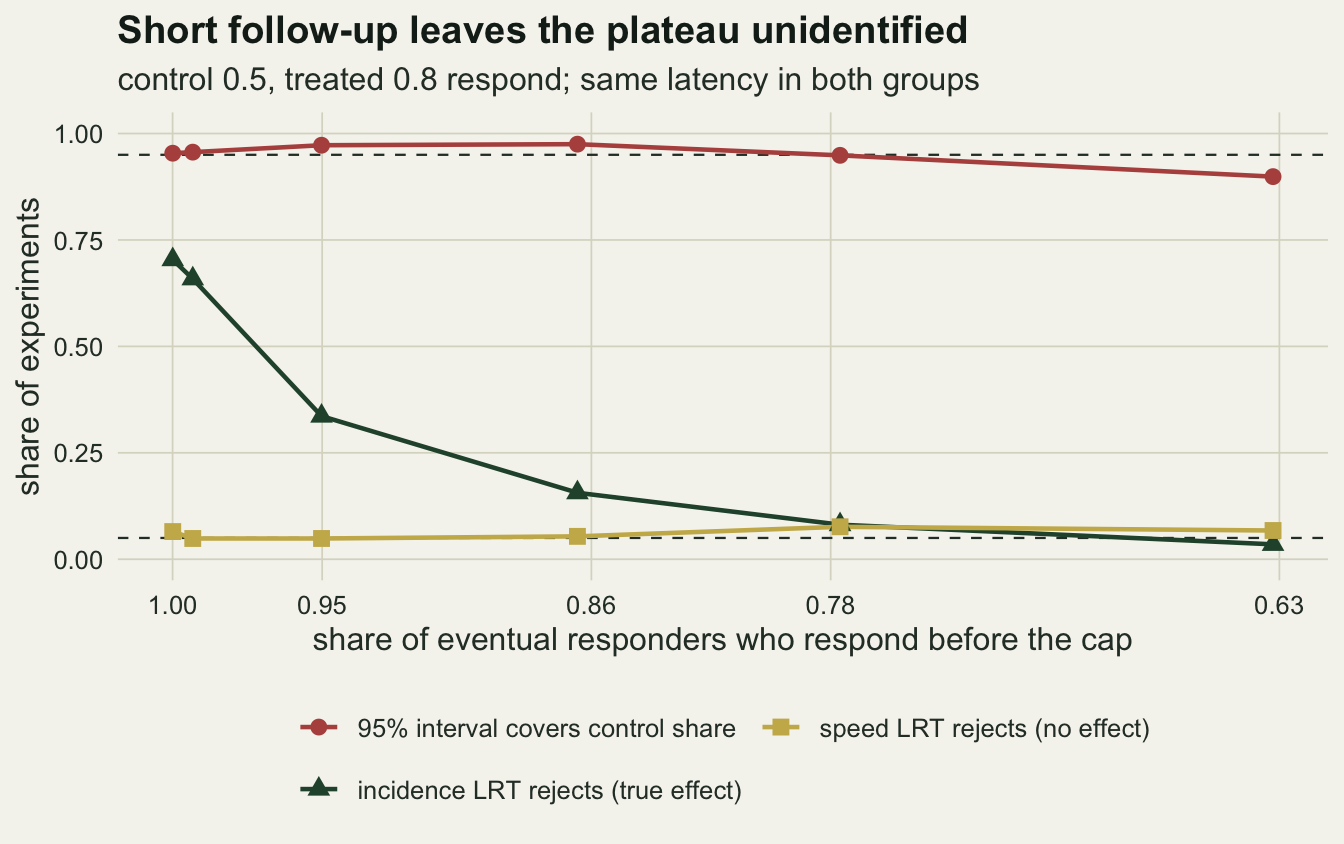
What to report
Report the cap and the number of animals that did not respond in each group, before any test. That table is the incidence half of the result, and in the faster-but-fewer scenario it points the opposite way from the latencies.
Plot the Kaplan-Meier curves to the cap and look at whether they flatten. A curve that levels off well above zero with no events in the last part of the trial is the sign of a non-responding fraction; a curve still falling at the cap is the sign of insufficient follow-up, and then the two effects cannot be separated from these data. A curve that looks flat is not enough: in the simulations the incidence test lost about half its power when 0.950 of responders had arrived before the cap. The check is a long censored stretch after the last observed return, long compared with the spread of the latencies that were observed.
Do not report a Cox hazard ratio as a speed effect when there is a plateau. In the more-responders scenario the median hazard ratio was 2.20 with no change in speed, and the proportional hazards test flagged it in 0.127 of experiments, so a clean cox.zph() does not license the reading. If a single test is wanted, the log-rank or Cox test answers “does the treatment change the share still waiting over the trial”, which is a fair question as long as it is described that way.
When the question is which part changed, fit a cure model with a logistic part for responding and a latency part for the responders, and report both effects with intervals. Say which latency distribution was used and check it: the exponential version gave a false speed effect in 0.225 of null experiments when the real shape was 0.5. A Weibull latency brought that to 0.073, at a large cost in power for the speed effect; the semiparametric Cox latency of Sy and Taylor avoids choosing a shape at all, but it was not simulated here.
Choose the cap from pilot latencies so that nearly all responders respond before it. In these simulations the power of the incidence test fell from 0.659 to 0.336 when the share of responders arriving before the cap dropped from 0.993 to 0.950, and to 0.156 at 0.865.
Honest limits
The two-group mixture is sharp: an animal either never responds or has a latency from one distribution. Real non-response is graded. A bird that did not come in 300 s might have come in 20 minutes, and the “cure” in a latency test is always relative to a trial length and to a motivational state that can change on the day. The cure model estimates the share that would not respond within a much longer window under the assumed latency shape; it cannot certify permanent non-response, which is the tail problem of the parametric survival post in another form.
Every animal here is tested once, independently. Behavioural latencies are often repeated across days, with individual consistency (personality) and habituation, and a treatment can shift both the share of responsive days and the speed on those days. That needs random effects in both parts of the model, which was not simulated.
The latency shapes were exponential and Weibull, with one shape shared by both groups. A treatment that changes the shape of the latency distribution, for example by creating a subgroup of very fast responders, is a third kind of effect that neither the exponential nor the shared-shape Weibull model has a parameter for.
The likelihood ratio tests use the chi-squared reference. At 30 animals per group that was at most slightly liberal for the exponential model and more liberal for the Weibull model (0.085 in one null cell). The sample sizes were 20 to 120 animals per group for the leak check and 30 for everything else; power for the effect sizes chosen here is specific to them.
The Cox model and the other one-number tests were only run with an exponential latency and full follow-up. Their behaviour under a Weibull shape or a short cap was not measured, and how the Cox hazard ratio in the more-responders case moves with either was not checked.
References
Berkson J, Gage RP 1952 Journal of the American Statistical Association 47(259):501-515 (10.1080/01621459.1952.10501187)
Farewell VT 1982 Biometrics 38(4):1041-1046 (10.2307/2529885)
Jahn-Eimermacher A, Lasarzik I, Raber J 2011 Behavioural Brain Research 221(1):271-275 (10.1016/j.bbr.2011.03.007)
Sy JP, Taylor JMG 2000 Biometrics 56(1):227-236 (10.1111/j.0006-341X.2000.00227.x)