library(ggplot2)

te_paper  <- "#f5f4ee"
te_ink    <- "#16241d"
te_body   <- "#2c3a31"
te_forest <- "#275139"
te_rust   <- "#b5534e"
te_gold   <- "#c9b458"
te_line   <- "#dad9ca"

theme_datasheet <- function() {
  theme_minimal(base_size = 12) +
    theme(plot.background  = element_rect(fill = te_paper, colour = NA),
          panel.background = element_rect(fill = te_paper, colour = NA),
          panel.grid.major = element_line(colour = te_line, linewidth = 0.3),
          panel.grid.minor = element_blank(),
          text             = element_text(colour = te_body),
          plot.title       = element_text(colour = te_ink, face = "bold"),
          plot.subtitle    = element_text(colour = te_body),
          axis.text        = element_text(colour = te_body))
}Activation energy and the rising limb
R
thermal ecology
physiology
nonlinear regression
simulation
ecology tutorial
With only high temperature deactivation, an Arrhenius slope fitted below the optimum still underestimates activation energy, by an amount set by Eh. In R.
A physiology lab measures the oxygen consumption of a ground beetle at fifteen temperatures, from 5 to 40 C in steps of 2.5 degrees, three beetles at each. The rate climbs steadily, peaks near 30 C and drops away above it. The number the lab wants is the activation energy E, the slope of log rate against minus one over Boltzmann’s constant times absolute temperature, because that is the number metabolic theory predicts and the number every comparison across species uses. The data above the peak are obviously not on a straight line, so the analyst does what the methods sections say: keep the rising limb, drop everything from a couple of degrees below the peak upwards, and fit the straight line to what is left.
That fix rests on an assumption that is rarely written down: that below the optimum the curve is still the pure Arrhenius exponential. In the model most people would reach for to describe the whole curve, the Sharpe-Schoolfield model with high temperature deactivation, it is not. The deactivating term starts to pull the curve down well before the peak, and how far below the peak its pull reaches depends on a second energy, the deactivation energy Eh, which the rising limb itself says very little about. With deactivation at the hot end only, the error this causes in the slope is always downwards; a low temperature deactivation can pull the cold end of the limb the other way, which a later section shows without noise but does not simulate. Pawar and colleagues (2016) showed with theory and more than a thousand thermal responses that activation energy estimates vary simply because studies measure different temperature ranges. This post reproduces that mechanism on one known curve and then measures what the rising limb fix and the whole curve fix each cost.
The moral that a monotone rate model breaks when the data reach the optimum is already on this site. The section “What thermal time cannot do” in Degree days and thermal time in R calibrates a linear degree day model to a development rate that bends down past its optimum, shows the prediction running early in a hot year, and ends with the repair: a nonlinear rate model fitted to the whole curve. That argument is not repeated here. The question here is the one it leaves open: whether staying below the optimum is enough. Thermal performance curves in R fits a Briere and a Gaussian curve and reads off the optimum, the upper limit and the breadth, but never an exponent; Checking a thermal performance analysis checks the extrapolated upper limit, the curve family and error in body temperature, and lists Schoolfield and colleagues (1981) only as a reference. Partitioning net flux into GPP and respiration finds its Lloyd-Taylor temperature sensitivity inflated, but by seasonal confounding in the basal rate, which is a different mechanism pushing in the opposite direction.
The structure follows Light response curves: the curvature you drop, which has the same shape of problem for a different curve. The bias from the rising limb fit is computed first, without noise, because it is an ordinary least squares slope through a known curve and no simulation is needed to find it. Then noise goes in: whether three replicates per temperature show the bend, what happens to the interval as replication grows, and what the Sharpe-Schoolfield fit through the peak costs.
A curve that turns over
The Sharpe-Schoolfield model with high temperature deactivation only writes the rate at absolute temperature T as an Arrhenius term divided by one plus the odds that the rate-limiting enzyme is in its inactive state:
r(T) = r_ref exp(E/k (1/T_ref - 1/T)) / (1 + exp(Eh/k (1/Th - 1/T)))
Here k is Boltzmann’s constant in electronvolts per kelvin, E the activation energy, Eh the deactivation energy and Th the temperature at which half the enzyme is inactive. This is the simplified form used in thermal ecology and coded as sharpeschoolhigh_1981() in the rTPC package of Padfield and colleagues (2021); the original of Schoolfield and colleagues (1981) also carries a factor of T/298 from absolute reaction rate theory and a low temperature deactivation term, both dropped here. The code below works with the log rate and with x = 1/(k T_ref) - 1/(k T), minus one over kT shifted to zero at a reference of 15 C, so that the Arrhenius part is a straight line of slope E in x.
k_B <- 1.380649e-23 / 1.602176634e-19
stopifnot(abs(k_B - 8.617333262e-5) < 1e-13)

E_true <- 0.65
T_opt  <- 30
T_ref  <- 15
eh_grid <- c(1.5, 2, 3, 4, 6)

to_kelvin <- function(temp_c) temp_c + 273.15
x_arr     <- function(temp_c) 1 / (k_B * to_kelvin(T_ref)) - 1 / (k_B * to_kelvin(temp_c))
softplus  <- function(z) pmax(z, 0) + log1p(exp(-abs(z)))
log_rate  <- function(temp_c, lnr_ref, e_act, e_h, t_h)
  lnr_ref + e_act * x_arr(temp_c) -
    softplus(e_h / k_B * (1 / to_kelvin(t_h) - 1 / to_kelvin(temp_c)))
th_for <- function(e_h, e_act = E_true, t_opt = T_opt)
  1 / (1 / to_kelvin(t_opt) + k_B / e_h * log(e_act / (e_h - e_act))) - 273.15

rtpc_form <- function(temp, r_tref, e, eh, th, tref) {
  r_tref * exp(e / k_B * (1 / (tref + 273.15) - 1 / (temp + 273.15))) /
    (1 + exp(eh / k_B * (1 / (th + 273.15) - 1 / (temp + 273.15))))
}
form_gap <- max(abs(exp(log_rate(seq(0, 45, 0.5), 0, 0.65, 2, 33)) -
                    rtpc_form(seq(0, 45, 0.5), 1, 0.65, 2, 33, T_ref)))

th_tab   <- sapply(eh_grid, th_for)
t_fine   <- seq(0, 45, by = 0.001)
topt_num <- sapply(seq_along(eh_grid), function(i)
  t_fine[which.max(log_rate(t_fine, 0, E_true, eh_grid[i], th_tab[i]))])
topt_gap <- max(abs(topt_num - T_opt))

lab_temp  <- seq(5, 40, by = 2.5)
rise_temp <- lab_temp[lab_temp <= T_opt - 2]
fall_temp <- lab_temp[lab_temp >= T_opt]
ols_slope <- function(temp_c, lr) unname(coef(lm(lr ~ x_arr(temp_c)))[2])
fall_slope <- sapply(seq_along(eh_grid), function(i)
  -ols_slope(fall_temp, log_rate(fall_temp, 0, E_true, eh_grid[i], th_tab[i])))
Boltzmann’s constant is computed from the two exact SI constants, which gives \(8.617333262 \times 10^{-5}\) eV per kelvin; the rTPC source (version 1.1.0 on GitHub, which is not loaded here) hard-codes the rounded \(8.62 \times 10^{-5}\). With the same constant in both, the log-scale function above and a direct transcription of the rTPC formula agree to within floating-point rounding over 0 to 45 C.
Setting the derivative of the log rate to zero gives the optimum in closed form. The local slope in x is E minus Eh times the logistic function of Eh/k (1/Th - 1/T), so the peak is where that logistic term equals E/Eh, which needs Eh above E and gives 1/Th = 1/T_opt + (k/Eh) log(E/(Eh - E)). The simulation fixes the optimum at 30 C for every curve and solves for Th, so that curves with different Eh share their peak and the same temperatures count as the rising limb. A numerical search on a grid of a thousandth of a degree finds every peak at 30 C, the largest gap being 0.000 degrees. The resulting Th runs from 31.4 to 33.4 C.
The activation energy is fixed at 0.65 eV. Dell and colleagues (2011) compiled 1,072 thermal responses and report a mean activation energy of 0.66 eV for the rising parts of within-species responses, with a right-skewed distribution around a median of 0.55, and a mean of 1.15 eV for the falling parts, which are right-skewed as well. That second number is not Eh. Well above Th the log rate falls with slope E - Eh in x, but a straight line fitted to the falling points of this design, 30 to 40 C, is much shallower, because the fall only reaches that asymptote far past the peak: it gives 0.32, 0.57, 1.18, 1.92 and 3.63 eV for Eh of 1.5, 2.0, 3.0, 4.0 and 6. A fall of 1.15 eV measured over those temperatures sits near Eh = 3. How far past the peak the published falls were measured varies between studies, so the grid is an assumption informed by Dell and colleagues, not a distribution taken from them; it runs from falls much gentler than their mean, the side on which a right-skewed distribution usually has its median, to much steeper ones.
t_plot <- seq(0, 42, by = 0.1)
curve_df <- do.call(rbind, lapply(seq_along(eh_grid), function(i)
  data.frame(x = x_arr(t_plot), lr = log_rate(t_plot, 0, E_true, eh_grid[i], th_tab[i]),
             eh = sprintf("Eh %.1f eV", eh_grid[i]))))
curve_df$eh <- factor(curve_df$eh, levels = sprintf("Eh %.1f eV", eh_grid))
temp_marks <- c(5, 15, 25, 30, 40)

ggplot(curve_df, aes(x, lr, colour = eh)) +
  annotate("rect", xmin = x_arr(min(rise_temp)), xmax = x_arr(max(rise_temp)),
           ymin = -Inf, ymax = Inf, fill = te_line, alpha = 0.6) +
  geom_abline(intercept = 0, slope = E_true, linetype = "dashed",
              colour = te_ink, linewidth = 0.6) +
  geom_line(linewidth = 0.9) +
  scale_colour_manual(values = c(te_rust, te_gold, te_forest, "#6d8f7a", te_ink),
                      name = NULL) +
  scale_x_continuous(sec.axis = sec_axis(~ ., breaks = x_arr(temp_marks),
                                         labels = temp_marks,
                                         name = "temperature (C)")) +
  coord_cartesian(ylim = c(-2.2, 2.2)) +
  labs(x = "x = 1/(k T_ref) - 1/(k T), per eV", y = "log rate relative to the Arrhenius rate at 15 C",
       title = "Five curves, one activation energy",
       subtitle = "grey band: the rising limb kept by the fix, 5 to 27.5 C") +
  theme_datasheet() +
  theme(legend.position = "bottom")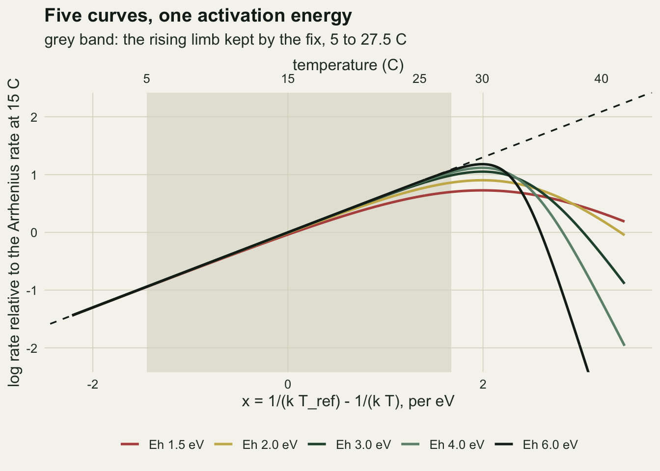
The rising-limb slope is arithmetic
Take the noise away and fit the straight line to the exact log rates at the rising limb temperatures. The answer is a fixed number for each curve: an ordinary least squares slope through known points. It needs no simulation and is not presented as a finding. What it shows is where the number comes from.
cut_temp <- lab_temp[lab_temp >= 15]
cut_tab <- do.call(rbind, lapply(seq_along(eh_grid), function(i)
  data.frame(e_h = eh_grid[i], cut = cut_temp,
             e_hat = sapply(cut_temp, function(cc) {
               tt <- lab_temp[lab_temp <= cc]
               ols_slope(tt, log_rate(tt, 0, E_true, eh_grid[i], th_tab[i]))
             }))))
rise_hat  <- cut_tab$e_hat[cut_tab$cut == max(rise_temp)]
rise_bias <- 100 * (rise_hat / E_true - 1)
low_cut   <- 20
low_hat   <- cut_tab$e_hat[cut_tab$cut == low_cut]
low_bias  <- 100 * (low_hat / E_true - 1)
full_hat  <- cut_tab$e_hat[cut_tab$cut == max(lab_temp)]

local_slope <- function(temp_c, e_h, t_h)
  E_true - e_h * plogis(e_h / k_B * (1 / to_kelvin(t_h) - 1 / to_kelvin(temp_c)))
slope_top <- sapply(seq_along(eh_grid), function(i) local_slope(max(rise_temp), eh_grid[i], th_tab[i]))
slope_bot <- sapply(seq_along(eh_grid), function(i) local_slope(min(rise_temp), eh_grid[i], th_tab[i]))
slope_mid <- sapply(seq_along(eh_grid), function(i) local_slope(low_cut, eh_grid[i], th_tab[i]))
n_low     <- sum(lab_temp <= low_cut)

x_r   <- x_arr(rise_temp)
lr_r  <- log_rate(rise_temp, 0, E_true, eh_grid[2], th_tab[2])
dev_r <- -cumsum(x_r - mean(x_r))[-length(x_r)] * diff(x_r)
sec_w <- dev_r / sum(dev_r)
sec_s <- diff(lr_r) / diff(x_r)
sec_gap <- abs(sum(sec_w * sec_s) - rise_hat[2])
stopifnot(all(sec_w > 0), sec_gap < 1e-12)

lr_q  <- function(temp_c) log_rate(temp_c, 0, E_true, eh_grid[2], th_tab[2])
q10_lo  <- exp(lr_q(20) - lr_q(10)); q10_hi <- exp(lr_q(30) - lr_q(20))
q10_arr <- exp(E_true / k_B * (1 / to_kelvin(10) - 1 / to_kelvin(20)))
q10_arr_hi <- exp(E_true / k_B * (1 / to_kelvin(20) - 1 / to_kelvin(30)))

# full Schoolfield denominator: 1 + cold odds + hot odds, on the log scale
lse3 <- function(a, b) { m <- pmax(0, a, b); m + log(exp(-m) + exp(a - m) + exp(b - m)) }
log_rate_lh <- function(temp_c, e_h, t_h, e_l, t_l)
  E_true * x_arr(temp_c) - lse3(e_l / k_B * (1 / to_kelvin(temp_c) - 1 / to_kelvin(t_l)),
                                e_h / k_B * (1 / to_kelvin(t_h) - 1 / to_kelvin(temp_c)))
e_low <- 2; t_low <- 2
cold_hat <- sapply(seq_along(eh_grid), function(i)
  ols_slope(rise_temp, log_rate_lh(rise_temp, eh_grid[i], th_tab[i], e_low, t_low)))
cold_top <- sapply(seq_along(eh_grid), function(i)
  t_fine[which.max(log_rate_lh(t_fine, eh_grid[i], th_tab[i], e_low, t_low))])
cold_drop5 <- 1 - exp(log_rate_lh(5, eh_grid[5], th_tab[5], e_low, t_low) -
                      log_rate(5, 0, E_true, eh_grid[5], th_tab[5]))
stopifnot(max(abs(cold_top - T_opt)) < 0.05, all(cold_hat[-1] > E_true), cold_hat[1] < E_true)
Fitted to the ten temperatures from 5 to 27.5 C, two degrees and more below the optimum, the slope is 0.543, 0.593, 0.628, 0.640 and 0.647 eV for Eh from 1.5 to 6, against a true 0.65. That is 16.5, 8.8, 3.4, 1.6 and 0.5 per cent low. At the Eh whose fall matches the mean of Dell and colleagues the fix loses 3.4 per cent; one step gentler, at Eh 2, it loses 8.8. The fit through all fifteen temperatures, peak and fall included, gives values from -0.071 to 0.328, which is the degree day post’s lesson in another form.
For this model the sign is guaranteed, and the reason is short. For sorted x the least squares slope is a weighted average of the slopes between neighbouring points, with weights proportional to minus the running sum of the deviations x - mean(x) times the gap to the next point, all of them positive; the chunk rebuilds the Eh 2 slope that way and matches lm() to within the chunk’s tolerance of \(10^{-12}\). Every neighbour slope is the local slope somewhere between the two points, and the local slope, E minus Eh times a logistic term, is below E at every temperature. So a straight line through any part of this curve returns less than E, whatever the cut.
That argument needs the local slope to stay at or below E everywhere in the kept range, which holds because this model deactivates only at the hot end. The full model of Schoolfield and colleagues (1981) adds a low temperature deactivation with its own energy and half-inactivation temperature, and its term adds to the local slope at the cold end instead of subtracting. The chunk puts an illustrative cold term on the same five curves, half inactive at 2 C with an energy of 2 eV (chosen, not taken from data), which lowers the rate at 5 C by 29 per cent and leaves every peak within a twentieth of a degree of 30 C. The noise-free slope from 5 to 27.5 C becomes 0.627 at Eh 1.5, still below E, but 0.678, 0.713, 0.725 and 0.732 from Eh 2 to 6, all above it. With deactivation at both ends the sign is not guaranteed. Pawar and colleagues (2016) report an upward direction across studies as well: when responses depart systematically from the Boltzmann-Arrhenius model, differences in measured range across studies can bias the distribution of activation energies towards a higher mean. Everything below uses the hot end term only, so its downward errors are the errors of that model, not a general rule.
How much less is set by how fast the logistic term dies away below the peak, and that rate is Eh. At the top of the kept range, 27.5 C, the local slope is 0.167 eV for Eh 1.5 and 0.544 for Eh 6; at 5 C it is 0.643 and 0.650. Ten degrees below the peak, at 20 C, the local slope is still 0.504 for Eh 1.5 but 0.650 for Eh 6. A gentle deactivation reaches far down the limb; a steep one leaves it straight until the last few degrees. Moving the cut further down therefore helps, but slowly: keeping only 5 to 20 C, ten degrees below the peak, still leaves the slope 6.6 per cent low at Eh 1.5 and 2.2 per cent at Eh 2, from 7 of the fifteen temperatures.
The same bend shows up in the everyday Q10. On the Eh 2 curve the rate rises by a factor of 2.40 from 10 to 20 C and 1.63 from 20 to 30 C, against 2.48 and 2.34 for the pure Arrhenius term over the same two intervals. A Q10 is a secant slope, and it inherits the deficit of the interval it spans.
cut_tab$eh <- factor(sprintf("Eh %.1f eV", cut_tab$e_h), levels = sprintf("Eh %.1f eV", eh_grid))
ggplot(cut_tab, aes(cut, e_hat, colour = eh)) +
  geom_hline(yintercept = E_true, linetype = "dashed", colour = te_ink, linewidth = 0.6) +
  geom_vline(xintercept = c(T_opt - 2, T_opt), linetype = "dotted",
             colour = te_body, linewidth = 0.5) +
  geom_line(linewidth = 0.9) +
  geom_point(size = 1.8) +
  scale_colour_manual(values = c(te_rust, te_gold, te_forest, "#6d8f7a", te_ink),
                      name = NULL) +
  labs(x = "highest temperature kept (C)", y = "fitted activation energy (eV)",
       title = "Every cut returns less than E",
       subtitle = "no noise, hot end deactivation only: least squares, lab grid from 5 C") +
  theme_datasheet() +
  theme(legend.position = "bottom")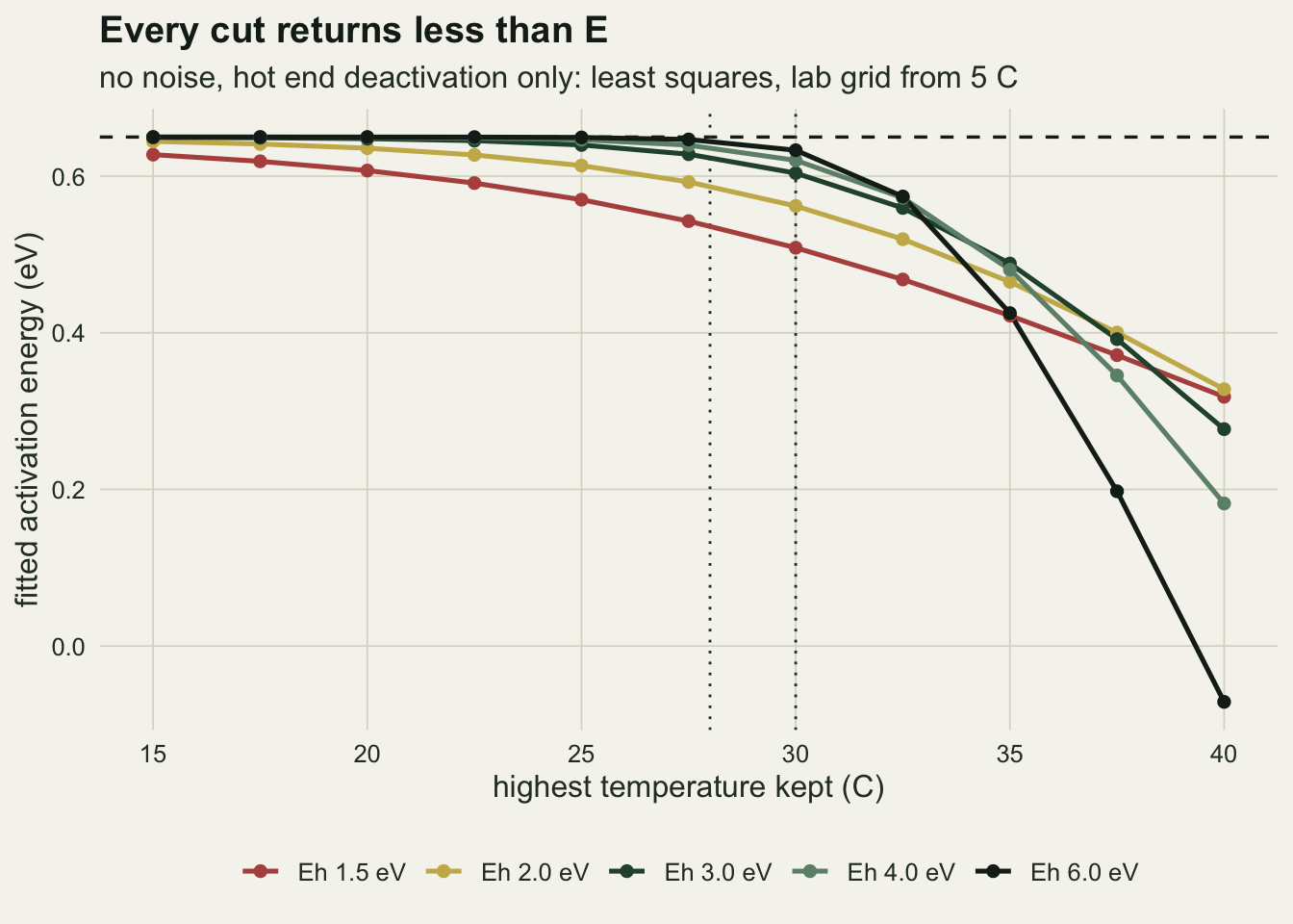
Three replicates do not show the bend
If the rising limb looked curved, an analyst would notice and cut lower. The design has replicates, so the natural check is the pure error lack-of-fit test: the spread of the temperature means about the straight line, against the spread of the replicates about their means. Under normal noise on the log scale that F statistic has a noncentral F distribution whose noncentrality is the replicate count times the noise-free lack-of-fit sum of squares divided by the noise variance, so its power is a closed form too. The noise is a lognormal with a standard deviation of 0.3 on the log scale, fixed before anything was run; the simulation below checks the closed form and supplies the interval coverage of the next section from the same draws.
sd_log   <- 0.3
rep_grid <- c(2, 3, 10, 30)
eh_mc    <- c(1.5, 2, 3, 6)
n_mc     <- 5000

mc_cell <- function(e_h, n_per) {
  tt    <- rep(rise_temp, each = n_per)
  n_obs <- length(tt)
  m_lev <- length(rise_temp)
  X     <- cbind(1, x_arr(tt))
  H     <- X %*% solve(crossprod(X), t(X))
  G     <- outer(tt, rise_temp, "==") * 1
  H_g   <- G %*% t(G) / n_per
  mu    <- log_rate(tt, 0, E_true, e_h, th_for(e_h))
  w_slope <- solve(crossprod(X), t(X))[2, ]
  f_crit  <- qf(0.95, m_lev - 2, n_obs - m_lev)
  ncp_lof <- sum(((H_g - H) %*% mu)^2) / sd_log^2
  bias    <- sum(w_slope * mu) - E_true
  se_true <- sd_log * sqrt(sum(w_slope^2))
  y_mat   <- mu + matrix(rnorm(n_obs * n_mc, 0, sd_log), n_obs)
  e_hat   <- colSums(w_slope * y_mat)
  ss_lof  <- colSums(((H_g - H) %*% y_mat)^2)
  ss_pe   <- colSums((y_mat - H_g %*% y_mat)^2)
  se_hat  <- sqrt((ss_lof + ss_pe) / (n_obs - 2) * sum(w_slope^2))
  covered <- abs(e_hat - E_true) <= qt(0.975, n_obs - 2) * se_hat
  f_stat  <- (ss_lof / (m_lev - 2)) / (ss_pe / (n_obs - m_lev))
  df_res <- n_obs - 2; t_q <- qt(0.975, df_res); d_std <- bias / se_true
  w_lim  <- qchisq(c(1e-12, 1 - 1e-12), df_res, ncp = ncp_lof)
  dens   <- function(w) dchisq(w, df_res, ncp = ncp_lof)
  cov_w  <- function(w) pnorm(t_q * sqrt(w / df_res) - d_std) - pnorm(-t_q * sqrt(w / df_res) - d_std)
  stopifnot(abs(integrate(dens, w_lim[1], w_lim[2], rel.tol = 1e-10)$value - 1) < 1e-8)
  cov_ex <- integrate(function(w) cov_w(w) * dens(w), w_lim[1], w_lim[2], rel.tol = 1e-10)$value
  fit_one <- lm(y_mat[, 1] ~ x_arr(tt))
  stopifnot(abs(coef(fit_one)[[2]] - e_hat[1]) < 1e-10,
            abs(sqrt(vcov(fit_one)[2, 2]) - se_hat[1]) < 1e-10)
  data.frame(e_h = e_h, n_per = n_per, bias = bias, se_true = se_true,
             pow_cf = pf(f_crit, m_lev - 2, n_obs - m_lev, ncp = ncp_lof, lower.tail = FALSE),
             pow_sim = mean(f_stat > f_crit),
             cov_cf = pnorm(qnorm(0.975) - d_std) - pnorm(-qnorm(0.975) - d_std),
             cov_t = pnorm(t_q - d_std) - pnorm(-t_q - d_std), cov_ex = cov_ex,
             cov_sim = mean(covered), above = mean(e_hat > E_true),
             mean_hat = mean(e_hat), sd_hat = sd(e_hat))
}

set.seed(23140)
mc_tab <- do.call(rbind, lapply(eh_mc, function(e_h)
  do.call(rbind, lapply(rep_grid, function(n_per) mc_cell(e_h, n_per)))))
mc_tab$pow_se <- sqrt(mc_tab$pow_sim * (1 - mc_tab$pow_sim) / n_mc)
mc_tab$cov_se <- sqrt(mc_tab$cov_sim * (1 - mc_tab$cov_sim) / n_mc)
pow_gap <- max(abs(mc_tab$pow_sim - mc_tab$pow_cf) / pmax(mc_tab$pow_se, 1e-3))
mc_row  <- function(e_h, n_per) mc_tab[mc_tab$e_h == e_h & mc_tab$n_per == n_per, ]
pow3_max <- max(mc_tab$pow_sim[mc_tab$n_per == 3])
pow6_rng <- range(mc_tab$pow_sim[mc_tab$e_h == 6])
se_max  <- sqrt(0.25 / n_mc)
cov_gap <- max(abs(mc_tab$cov_sim - mc_tab$cov_ex) / pmax(mc_tab$cov_se, 1e-3)); stopifnot(cov_gap < 4)
t_share <- with(mc_row(1.5, 3), (cov_t - cov_cf) / (cov_ex - cov_cf)); stopifnot(t_share > 0.5, t_share < 1)
Each cell has 5000 simulated experiments, so the Monte Carlo standard error of any rate is at most 0.0071. The simulated rejection rates sit within 1.8 Monte Carlo standard errors of the noncentral F values in every cell, and the chunk checks the matrix route against lm() on one data set.
With three beetles per temperature the test rejects the straight line in 0.075 of experiments at Eh 1.5, where the fix loses 16.5 per cent of E, and in 0.062 at Eh 2. The level of the test is 0.05, so at usual replication the bend that biases the slope is close to invisible. The test does get there with effort: at 30 per temperature its power is 0.63 at Eh 1.5 and 0.32 at Eh 2. At Eh 3 and 30 per temperature it is 0.11, and at Eh 6 it stays between 0.048 and 0.057 at every replication, as it should when the kept limb is nearly straight. This is the practical meaning of saying the rising limb cannot tell you Eh: the only information about the deactivation energy on the rising limb is its curvature, and three replicates at noise of this size cannot see it.
More replicates make the interval worse
The least squares slope on the rising limb is exactly normal here, centred on the noise-free slope computed in “The rising-limb slope is arithmetic” with a standard deviation that shrinks as one over the square root of the replicate count. The bias does not shrink. So the ratio of bias to standard error grows like the square root of the replication, and the coverage of the nominal 95 per cent interval falls towards zero. That is arithmetic again: with the noise level known, coverage is the normal probability Phi(1.96 - b/se) - Phi(-1.96 - b/se). The interval lm() reports differs in two ways: it uses a t quantile on n - 2 degrees of freedom, and it estimates the residual variance, which the lack of fit inflates. Its coverage is still a closed form. The slope is independent of the residual sum of squares, and that sum divided by the noise variance has a noncentral chi-square distribution with the lack-of-fit noncentrality of the previous section, so the coverage is the normal probability with the t quantile scaled by the square root of that ratio over its degrees of freedom, averaged over the ratio’s distribution. The chunk does the averaging with integrate() between the \(10^{-12}\) and \(1 - 10^{-12}\) quantiles of the noncentral chi-square, checks that the density integrates to one between them, and compares the result with the simulated coverage.
At Eh 1.5 the interval covers the true E in 0.694 of experiments with two beetles per temperature, 0.542 with three, 0.062 with ten and in 0 of 5000 with thirty. At Eh 2 the same four values are 0.879, 0.830, 0.545 and 0.090; at Eh 3 they are 0.938, 0.937, 0.892 and 0.758; at Eh 6 they stay between 0.945 and 0.951. The Monte Carlo standard errors are at most 0.0070. The exact coverage of the lm() interval is within 1.2 Monte Carlo standard errors of the simulated rate in every cell. For Eh 1.5 and three per temperature it is 0.545 against the simulated 0.542; the normal formula with the noise known gives 0.503, and the t quantile alone, still with the noise known, 0.538. Of the gap between the normal formula and the exact value, 84 per cent is the t quantile; the estimated and inflated variance adds the rest.
Put the two panels of the next figure side by side and the order of events is clear. By the time replication is high enough for the lack-of-fit test to see the bend with reasonable power, the interval around the rising limb slope has stopped covering the truth. A larger experiment does not rescue a misspecified model; it reports the wrong number with more confidence.
plot_mc <- rbind(
  data.frame(e_h = mc_tab$e_h, n_per = mc_tab$n_per, value = mc_tab$cov_sim,
             se = mc_tab$cov_se, panel = "interval covers the true E"),
  data.frame(e_h = mc_tab$e_h, n_per = mc_tab$n_per, value = mc_tab$pow_sim,
             se = mc_tab$pow_se, panel = "lack-of-fit test rejects the line"))
plot_mc$eh <- factor(sprintf("Eh %.1f eV", plot_mc$e_h), levels = sprintf("Eh %.1f eV", eh_mc))
ref_mc <- data.frame(panel = c("interval covers the true E", "lack-of-fit test rejects the line"),
                     yref = c(0.95, 0.05))

ggplot(plot_mc, aes(n_per, value, colour = eh)) +
  geom_hline(data = ref_mc, aes(yintercept = yref), linetype = "dashed",
             colour = te_ink, linewidth = 0.5) +
  geom_line(linewidth = 0.9) +
  geom_errorbar(aes(ymin = value - 2 * se, ymax = value + 2 * se), width = 0.03,
                linewidth = 0.5) +
  geom_point(size = 2) +
  facet_wrap(~ panel, ncol = 2) +
  scale_x_log10(breaks = rep_grid) +
  scale_y_continuous(limits = c(0, 1)) +
  scale_colour_manual(values = c(te_rust, te_gold, te_forest, te_ink), name = NULL) +
  labs(x = "replicates per temperature (log scale)", y = "proportion of experiments",
       title = "The bend shows up after the interval has failed",
       subtitle = "rising limb 5 to 27.5 C, lognormal noise sd 0.3") +
  theme_datasheet() +
  theme(legend.position = "bottom",
        strip.text = element_text(colour = te_ink, face = "bold"))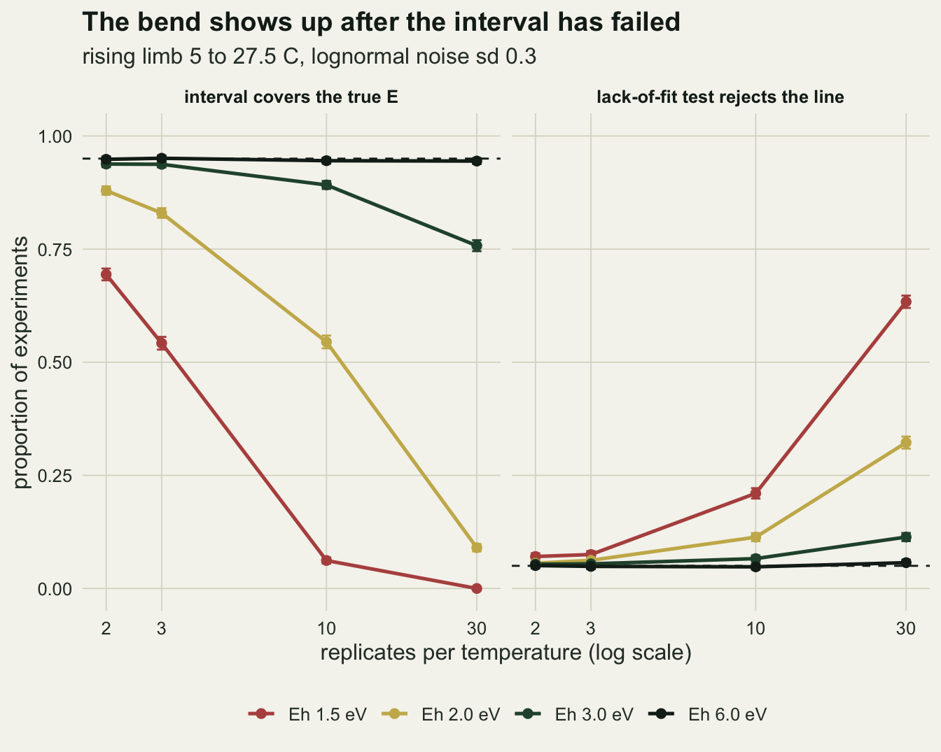
Fitting through the peak
The repair the degree day post names is to fit the nonlinear rate model to the whole curve, so the same simulated experiments now keep all fifteen temperatures and fit the four parameter Sharpe-Schoolfield model by nonlinear least squares on the log rate. Its likelihood can have more than one valley in Eh and Th, and a single fixed start is a known source of silent failure, so each fit starts from the best point of a grid. The model is linear in the log reference rate and in E once Eh and Th are fixed, so for each pair on a grid of 45 log spaced values of Eh from 0.8 to 20 eV and values of Th from 15 to 50 C in steps of 0.5 degrees the residual sum of squares comes from one matrix product, and nls() starts from the best pair. Replication is 500 data sets per cell at three and at ten beetles per temperature, and the rising limb fit is computed on the same data sets.
eh_start <- exp(seq(log(0.8), log(20), length.out = 45))
th_start <- seq(15, 50, by = 0.5)
pair_grid <- expand.grid(e_h = eh_start, t_h = th_start)
n_ss  <- 500
eh_ss <- c(1.5, 2, 3, 6)

ss_cell <- function(e_h, n_per) {
  tt    <- rep(lab_temp, each = n_per)
  n_obs <- length(tt)
  X     <- cbind(1, x_arr(tt))
  M     <- diag(n_obs) - X %*% solve(crossprod(X), t(X))
  off_mat <- sapply(seq_len(nrow(pair_grid)), function(j)
    -softplus(pair_grid$e_h[j] / k_B * (1 / to_kelvin(pair_grid$t_h[j]) - 1 / to_kelvin(tt))))
  m_off <- M %*% off_mat
  in_rise <- tt <= T_opt - 2
  mu <- log_rate(tt, 0, E_true, e_h, th_for(e_h))
  out <- t(replicate(n_ss, {
    ly  <- mu + rnorm(n_obs, 0, sd_log)
    j   <- which.min(colSums((as.vector(M %*% ly) - m_off)^2))
    b0  <- lm.fit(X, ly - off_mat[, j])$coefficients
    fit <- tryCatch(nls(ly ~ lnr + e_act * x_arr(tt) -
                          softplus(eh_fit / k_B * (1 / to_kelvin(th_fit) - 1 / to_kelvin(tt))),
                        start = list(lnr = b0[[1]], e_act = b0[[2]],
                                     eh_fit = pair_grid$e_h[j], th_fit = pair_grid$t_h[j])),
                    error = function(err) NULL)
    rise_fit <- lm(ly[in_rise] ~ x_arr(tt[in_rise]))
    rise_ci  <- confint(rise_fit)[2, ]
    edge <- pair_grid$e_h[j] %in% range(eh_start) || pair_grid$t_h[j] %in% range(th_start)
    if (is.null(fit)) c(NA, NA, coef(rise_fit)[[2]], rise_ci[1] <= E_true && E_true <= rise_ci[2], edge, NA)
    else c(coef(fit)[["e_act"]], sqrt(vcov(fit)["e_act", "e_act"]), coef(rise_fit)[[2]],
           rise_ci[1] <= E_true && E_true <= rise_ci[2], edge, coef(fit)[["eh_fit"]])
  }))
  ok <- !is.na(out[, 1])
  d_sq <- (out[ok, 1] - E_true)^2 - (out[ok, 3] - E_true)^2
  q_ss <- qt(0.975, n_obs - 4)
  list(summary = data.frame(e_h = e_h, n_per = n_per, n_ok = sum(ok), n_edge = sum(out[, 5]),
         ss_med = median(out[ok, 1]), ss_mean = mean(out[ok, 1]), ss_q1 = quantile(out[ok, 1], 0.25)[[1]],
         ss_q3 = quantile(out[ok, 1], 0.75)[[1]], ss_sd = sd(out[ok, 1]),
         ss_rmse = sqrt(mean((out[ok, 1] - E_true)^2)),
         ss_cov = mean(abs(out[ok, 1] - E_true) <= q_ss * out[ok, 2]),
         ss_width = median(2 * q_ss * out[ok, 2]),
         ri_mean = mean(out[, 3]), ri_sd = sd(out[, 3]),
         ri_rmse = sqrt(mean((out[ok, 3] - E_true)^2)), ri_cov = mean(out[, 4]),
         mse_diff = mean(d_sq), mse_diff_se = sd(d_sq) / sqrt(sum(ok)),
         cor_e_eh = cor(out[ok, 1], out[ok, 6])),
       draws = data.frame(e_h = e_h, n_per = n_per,
                          method = rep(c("Sharpe-Schoolfield, 5 to 40 C", "Arrhenius, 5 to 27.5 C"),
                                       c(sum(ok), n_ss)),
                          e_hat = c(out[ok, 1], out[, 3])))
}

set.seed(51077)
ss_runs <- lapply(eh_ss, function(e_h) lapply(c(3, 10), function(n_per) ss_cell(e_h, n_per)))
ss_tab  <- do.call(rbind, lapply(unlist(ss_runs, recursive = FALSE), `[[`, "summary"))
ss_draw <- do.call(rbind, lapply(unlist(ss_runs, recursive = FALSE), `[[`, "draws"))
ss_row  <- function(e_h, n_per) ss_tab[ss_tab$e_h == e_h & ss_tab$n_per == n_per, ]
cov_se_ss <- sqrt(ss_tab$ss_cov * (1 - ss_tab$ss_cov) / ss_tab$n_ok)
stopifnot(sum(ss_tab$n_edge) == ss_row(1.5, 3)$n_edge)
mean_gap <- ss_tab$ss_mean - E_true; z_mse <- ss_tab$mse_diff / ss_tab$mse_diff_se
stopifnot(which.max(mean_gap) == which(ss_tab$e_h == 1.5 & ss_tab$n_per == 3))
Of the 4000 fits, 3998 converged, and 6 started from the edge of the start grid, all of them at Eh 1.5 with three per temperature. Through the peak the activation energy comes back without the systematic loss: with three beetles per temperature the median estimate is 0.671, 0.654, 0.653 and 0.647 for Eh 1.5, 2, 3 and 6. The means are 0.696, 0.657, 0.658 and 0.650: at the gentlest fall the distribution has a long upper tail and the mean sits above the truth. The nominal 95 per cent Wald interval from nls() covers the true E in 0.930, 0.940, 0.952 and 0.960 of fits (Monte Carlo standard error at most 0.011). At ten per temperature the coverages are 0.930, 0.962, 0.950 and 0.966.
The price is spread, and it is highest exactly where the fix is most needed. At three per temperature and Eh 1.5 the Sharpe-Schoolfield estimates have a standard deviation of 0.164 and an interquartile range of 0.588 to 0.771, against 0.056 for the rising limb slope, whose mean is 0.545. At Eh 6 the two standard deviations are 0.050 and 0.054. With the gentler falls the fitted E and Eh are more strongly tied than with the steepest: across fits at three per temperature their correlation is -0.37, -0.59 and -0.43 for Eh 1.5, 2 and 3, against -0.19 at Eh 6.
That spread has a consequence worth stating plainly. Measured by root mean square error at three per temperature, the biased rising limb slope is the more accurate number at Eh 1.5: 0.119 against 0.170, a difference in mean squared error of 0.0147 with a paired Monte Carlo standard error of 0.0035, while its interval covers the truth in 0.566 of these 500 data sets (0.542 over the 5000 of the previous section). At Eh 2 the two are indistinguishable at this replication (0.083 against 0.089, difference 0.0010, standard error 0.0007). At ten per temperature the order is reversed: 0.077 for Sharpe-Schoolfield against 0.112 at Eh 1.5, and 0.046 against 0.062 at Eh 2, both differences at least 9 paired standard errors from zero, and the whole curve interval covers in 0.930 and 0.962 against 0.054 and 0.596. At Eh 3 and 6 the two errors are close at ten per temperature: 0.033 against 0.037 and 0.026 against 0.027, 3.1 and 2.2 paired standard errors apart; what still separates them at Eh 3 is coverage, 0.950 against 0.892. With a small experiment and a gentle fall the choice is between a tighter number that is wrong by an unknown amount and a looser one whose interval means what it says; with a larger experiment and a gentle fall the whole curve fit wins on both counts, and at the steepest fall the two are close on both.
ss_draw$eh <- factor(sprintf("Eh %.1f", ss_draw$e_h), levels = sprintf("Eh %.1f", eh_ss))
ss_draw$reps <- factor(sprintf("%d per temperature", ss_draw$n_per),
                       levels = sprintf("%d per temperature", c(3, 10)))
n_clip <- sum(ss_draw$e_hat < 0.3 | ss_draw$e_hat > 1.2)
ggplot(ss_draw, aes(eh, e_hat, fill = method)) +
  geom_hline(yintercept = E_true, linetype = "dashed", colour = te_ink, linewidth = 0.6) +
  geom_boxplot(outlier.size = 0.6, outlier.alpha = 0.4, width = 0.7,
               colour = te_body, linewidth = 0.4) +
  facet_wrap(~ reps, ncol = 2) +
  scale_fill_manual(values = c(te_rust, te_forest), name = NULL) +
  coord_cartesian(ylim = c(0.3, 1.2)) +
  labs(x = "deactivation energy (eV)", y = "estimated activation energy (eV)",
       title = "Through the peak: wider, and centred near E",
       subtitle = sprintf("%d experiments per box; %d estimates outside 0.3 to 1.2 not drawn",
                         n_ss, n_clip)) +
  theme_datasheet() +
  theme(legend.position = "bottom",
        strip.text = element_text(colour = te_ink, face = "bold"))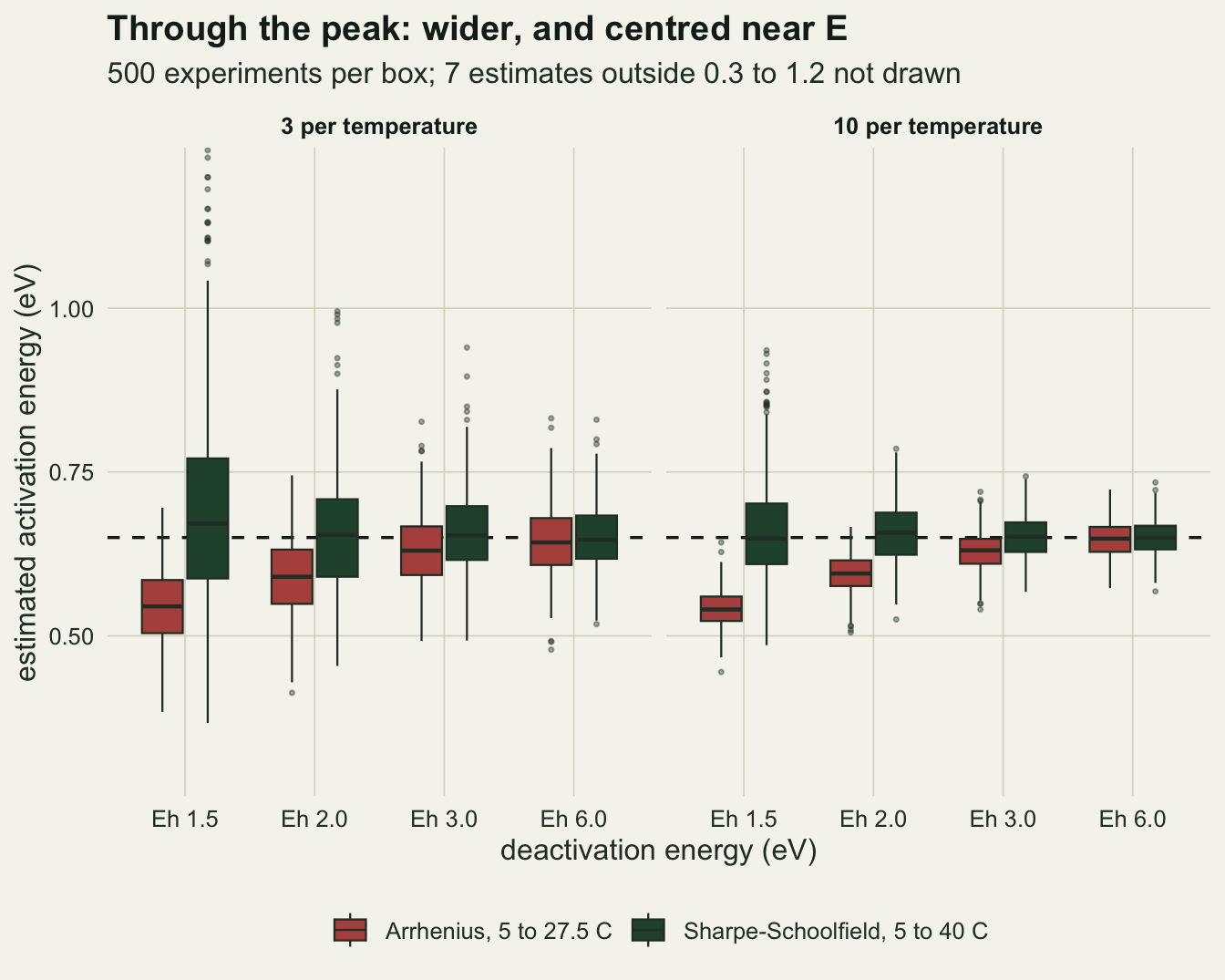
What to report
Report the temperature range an activation energy was fitted over, and say how the range was chosen. A slope from a range cut two degrees below the apparent optimum estimates a weighted average of secants through the curve, not E. Under high temperature deactivation alone, as simulated here, that target is always below E; a low temperature deactivation pushes the cold end the other way, and then the sign is not guaranteed. How far the target sits from E depends on Eh, and on the cold term if there is one, and the rising limb estimates neither, so no correction that ignores them can be applied afterwards. Pawar and colleagues (2016) give guidelines and an equation for a partial correction; it was not tried here.
If the whole curve was measured, fit the whole curve. A Sharpe-Schoolfield fit through the peak had medians within 0.021 eV of the true E in every case above, with means up to 0.046 eV above it (Eh 1.5, three per temperature) from a long upper tail; its interval covered in 0.930 to 0.966 of fits, with 4 temperatures above the optimum in the data. Start nls() from a grid over Eh and Th, or from several starts as the rTPC and nls.multstart pipeline does, and report Eh and Th alongside E, because a wide interval on E goes with a gentle fall in which E and Eh are hard to separate.
If only the rising limb exists, say so, and for a curve that deactivates only at the hot end treat the slope’s expected value as a lower bound on E, with an unknown gap. A single slope is not a bound: where the limb is nearly straight it lands above E almost as often as below, in 0.468 of experiments at Eh 6 with three per temperature. Do not quote its confidence interval as the uncertainty in E: at ten replicates per temperature it covered the true value in 54 per cent of experiments at Eh 2. A lack-of-fit test on the rising limb is worth running, but a non-significant one is not evidence that the limb is straight; at three per temperature it rejected in at most 0.075 of experiments at every Eh simulated.
Comparisons of E between species or treatments inherit all of this. Two species with the same activation energy and different deactivation energies return different rising limb slopes from identical protocols: here 0.543 and 0.647. A difference in E measured this way may be a difference in how sharply the two species fall.
Honest limits
The truth is the Sharpe-Schoolfield curve itself, so the whole curve fit is the correctly specified model here. Real curves can depart from it: a low temperature deactivation, a plateau, or a fall that is not an enzyme equilibrium at all. The Sharpe-Schoolfield fit was not tested against a truth from another family, and its good coverage above is coverage under its own model. For the rising limb fit the first of these can reverse the direction of the error: in the noise-free check above, the cold end term turned the downward bias into an upward one at 4 of the 5 values of Eh. Only one illustrative cold term was tried, without noise, and the whole curve fit was not run on it.
The rising limb was cut with the true optimum known. In a real experiment the cut is placed relative to the highest observed mean, which is itself noisy on a flat topped curve and can land on either side of the true optimum, moving the cut and the bias with it. That was not measured.
One activation energy, one optimum, one lab grid and one noise level were simulated. The bias table changes with all of them: a denser grid near the top of the kept range would put more weight on the most curved part, and the percentage losses above are for this grid and should be recomputed, not transferred. The Eh grid is an assumption bracketing the mean fall reported by Dell and colleagues under this design, not a sample from the distribution of real deactivation energies.
The noise is independent lognormal with constant variance on the log scale, and each beetle contributes one measurement. Repeated measurements of the same animals across temperatures, which is common in respirometry, would need a mixed model and change both intervals. Measurement error in temperature, which Checking a thermal performance analysis treats for the curve itself, was left out.
The Wald interval from nls() was the only whole curve interval examined, and only for E. Profile likelihood intervals were not tried, and nothing above says how the intervals for Eh and Th behave, which matters because at the gentlest fall the estimates of E have a long upper tail.
References
Schoolfield RM, Sharpe PJH, Magnuson CE 1981 Journal of Theoretical Biology 88(4):719-731 (10.1016/0022-5193(81)90246-0)
Dell AI, Pawar S, Savage VM 2011 Proceedings of the National Academy of Sciences 108(26):10591-10596 (10.1073/pnas.1015178108)
Pawar S, Dell AI, Savage VM, Knies JL 2016 The American Naturalist 187(2):E41-E52 (10.1086/684590)
Padfield D, O’Sullivan H, Pawar S 2021 Methods in Ecology and Evolution 12(6):1138-1143 (10.1111/2041-210X.13585)