library(ggplot2)

te_paper  <- "#f5f4ee"
te_ink    <- "#16241d"
te_body   <- "#2c3a31"
te_forest <- "#275139"
te_rust   <- "#b5534e"
te_gold   <- "#c9b458"
te_line   <- "#dad9ca"

theme_datasheet <- function() {
  theme_minimal(base_size = 12) +
    theme(plot.background  = element_rect(fill = te_paper, colour = NA),
          panel.background = element_rect(fill = te_paper, colour = NA),
          panel.grid.major = element_line(colour = te_line, linewidth = 0.3),
          panel.grid.minor = element_blank(),
          text             = element_text(colour = te_body),
          plot.title       = element_text(colour = te_ink, face = "bold"),
          plot.subtitle    = element_text(colour = te_body),
          axis.text        = element_text(colour = te_body))
}

p_sad   <- c(0.40, 0.30, 0.20, 0.10)
n_spec  <- length(p_sad)
h_true  <- -sum(p_sad * log(p_sad))
s_true  <- sum(p_sad^2)
n_grid  <- c(10, 20, 40, 80, 160)
n_short <- n_grid[2]
n_long <- n_grid[5]The jackknife and bias correction
R
resampling
statistics
diversity
ecology tutorial
The jackknife removes bias, it does not build intervals. See its pseudo-values cancel the one over n term in a diversity index, and then fail on a median in R.
Two pitfall plots in the same beech stand, the same four ground beetle species underneath both of them, and a technician who emptied one set of traps after a fortnight and the other after a full season. The short plot yields twenty beetles, the long one yields one hundred and sixty. Both get a Shannon index, and the long plot comes out more diverse.
Nothing about the community differs. The index is a function of proportions, the proportions are estimated from counts, and the plug-in index computed from estimated proportions sits below the index of the community it came from. The shortfall shrinks as the sample grows, which is exactly what makes it dangerous: an effort gradient across plots turns into a diversity gradient, in the direction field ecologists usually expect to see.
This is the problem the jackknife was built for. Quenouille proposed deleting one observation at a time, recomputing, and combining the results so that the leading term of the bias cancels; Tukey turned the recomputations into pseudo-values and gave the method its name, and Miller’s review two decades later gathered both halves of it, the bias correction and the variance estimate, into one account, with the conditions the variance half needs already spelled out. What it removes is a bias of order one over the sample size, which is nearly always the leading term of the bias of a plug-in estimator. The site has used the jackknife as a variance device in five posts, and in none of those five for bias correction. It supplies the acceleration term of a BCa interval in the nonparametric bootstrap, and a delete-one standard error in the Deming regression post, the effective size post, the acoustic checking post and the calibration overlap post. It appears in two further posts as a formula, and those two are bias corrections: the first and second order jackknife richness estimators in asymptotic richness estimators, and the jackknife abundance estimator in capture heterogeneity, both quoted without the delete-one argument that produces them. A bias correction device used as a variance tool, or as a formula with its derivation left out.
This post measures what it was built to do, and where it stops. Checking a bootstrap already states the general rule that resampling needs a statistic that is smooth in the data, and extends it from the sample maximum to minima, ranges and boundary parameters. The result below runs that rule backwards. The median is smooth enough for the bootstrap and not smooth enough for the jackknife, at the same sample sizes, so smoothness is not one property that resampling methods either have or lack. The jackknife needs more of it, and no sample size repairs the shortfall.
Two plots, one community, and an effort gradient
Four species with relative abundances of 0.40, 0.30, 0.20 and 0.10. The Shannon index of that community is 1.2799 and its Simpson concentration is 0.300. Both are fixed properties of the community, and both are what an estimator is trying to hit.
With only four species the whole sampling distribution can be written down. A sample of size 160 from four species has 708,561 possible count vectors, and every one of them has a multinomial probability, so the expected value of any estimator is a finite sum rather than something to simulate. Every bias quoted for the Shannon or Simpson index below is that sum, evaluated exactly. There is no Monte Carlo error in any of those numbers.
comps <- function(n_ind, n_sp) {
  parts <- matrix(0:n_ind, ncol = 1)
  if (n_sp > 2) for (k in 2:(n_sp - 1)) {
    rem <- n_ind - rowSums(parts)
    parts <- cbind(parts[rep(seq_len(nrow(parts)), rem + 1), , drop = FALSE],
                   unlist(lapply(rem, function(z) 0:z)))
  }
  unname(cbind(parts, n_ind - rowSums(parts)))
}

shannon_plug <- function(counts, tot) {
  prop <- counts / tot
  term <- prop * log(prop)
  term[!is.finite(term)] <- 0
  -rowSums(term)
}
simpson_plug <- function(counts, tot) rowSums((counts / tot)^2)

exact_pair <- function(n_ind, probs, stat) {
  counts <- comps(n_ind, length(probs))
  wt <- exp(lgamma(n_ind + 1) - rowSums(lgamma(counts + 1)) +
            as.vector(counts %*% log(probs)))
  plug <- stat(counts, n_ind)
  loo <- numeric(nrow(counts))
  for (j in seq_along(probs)) {
    drop_j <- counts
    drop_j[, j] <- pmax(drop_j[, j] - 1, 0)
    loo <- loo + (counts[, j] / n_ind) * stat(drop_j, n_ind - 1)
  }
  c(plug = sum(wt * plug),
    jack = sum(wt * (n_ind * plug - (n_ind - 1) * loo)),
    mass = sum(wt))
}

sh_tab <- t(vapply(n_grid, exact_pair, numeric(3), probs = p_sad,
                   stat = shannon_plug))
si_tab <- t(vapply(n_grid, exact_pair, numeric(3), probs = p_sad,
                   stat = simpson_plug))
bias <- data.frame(n = n_grid,
                   plug = sh_tab[, "plug"] - h_true,
                   jack = sh_tab[, "jack"] - h_true,
                   si_plug = si_tab[, "plug"] - s_true,
                   si_jack = si_tab[, "jack"] - s_true)
mass_err <- max(abs(sh_tab[, "mass"] - 1))
gap_effort <- bias$plug[5] - bias$plug[2]
The count vectors carry a total probability that departs from one by 9.2e-14, which is the arithmetic working. The short plot returns a Shannon index that sits on average 0.0812 below the truth, or 6.3 per cent of it. The long plot sits 0.0094 below, or 0.7 per cent. The gap between the two expectations is 0.0717 index units, and it is produced entirely by trapping effort.
The pseudo-values cancel the one over n term
Write the estimator computed from all 20 observations as one number and the estimator computed with observation i deleted as another. The delete-one values are averaged, and the jackknifed estimate is the full-sample value scaled up by the sample size minus the average of the delete-one values scaled up by one less. The pseudo-values are the same arithmetic written per observation, and the jackknifed estimate is their mean.
The algebra is short enough to follow. Suppose the expected value of the estimator at sample size n is the target plus a term in one over n plus a term in one over n squared. The delete-one estimators have expectation with n minus one in those denominators. Multiply the first by n, the second by n minus one, subtract, and the one over n terms cancel exactly, for any constant multiplying them. The one over n squared term does not cancel, and it survives multiplied by a factor of about one over n. That is the whole mechanism, and it says what the method can and cannot promise: the leading bias term goes, the next one shrinks.
jack_parts <- function(dat, stat) {
  n_obs <- length(dat)
  loo <- vapply(seq_len(n_obs), function(i) stat(dat[-i]), 0)
  pseudo <- n_obs * stat(dat) - (n_obs - 1) * loo
  list(loo = loo, pseudo = pseudo, est = mean(pseudo),
       var_jack = (n_obs - 1) / n_obs * sum((loo - mean(loo))^2))
}
plug_var <- function(dat) mean((dat - mean(dat))^2)

set.seed(4071)
mass_g <- rlnorm(20, log(28), 0.55)
n_mass <- length(mass_g)

jk_mean <- jack_parts(mass_g, mean)
jk_var  <- jack_parts(mass_g, plug_var)

id_pseudo <- max(abs(jk_mean$pseudo - mass_g))
id_varmean <- abs(jk_mean$var_jack - var(mass_g) / n_mass)
id_varjack <- abs(jk_var$est - var(mass_g))
id_pvar <- abs(var(jk_mean$pseudo) / n_mass - jk_mean$var_jack)
Three identities make the machinery concrete, and all three are exact rather than approximate. For the sample mean the pseudo-values are the observations themselves: the largest discrepancy over 20 beetle masses is 8.9e-14. The jackknife variance of the mean is the usual sample variance divided by the sample size, to 1.1e-14. And the jackknife applied to the plug-in variance, which divides by n, returns the ordinary variance that divides by n minus one, to 2.6e-13. The correction is not an approximation to the familiar denominator fix; it is that fix.
The link between the two halves of the method is the last identity: the variance of the pseudo-values divided by the sample size is the jackknife variance estimate, to 1.1e-14. Their mean corrects the bias and their scatter estimates the variance, from one set of 20 recomputations.
On a diversity index the correction removes most of the bias
The Simpson concentration is the cleanest case available, because its plug-in bias is exactly one minus the concentration, divided by the sample size, with nothing after it.
si_pred <- (1 - s_true) / n_grid
si_pred_err <- max(abs(bias$si_plug - si_pred))
si_jack_max <- max(abs(bias$si_jack))
sh_removed <- 100 * (1 - abs(bias$jack) / abs(bias$plug))
The predicted plug-in bias matches the enumerated one to 4.30e-14 at every sample size. Because the bias is a constant over n with no higher terms, the cancellation is complete rather than partial: across the five sample sizes the largest absolute bias of the jackknifed Simpson estimator is 4.12e-14, which is the noise floor of double precision arithmetic. Not small. Zero.
The Shannon index is the realistic case. Its plug-in bias, which Basharin worked out, starts at minus the number of species minus one, over twice the sample size, and then continues. The jackknife can only remove the first term.
sh_pred <- -(n_spec - 1) / (2 * n_grid)
sh_ratio <- bias$plug / sh_pred
sh_short_pc <- 100 * bias$plug[2] / h_true
sh_short_jk_pc <- 100 * bias$jack[2] / h_true
At the short plot’s sample size the plug-in index is biased by -6.3 per cent of the true index and the jackknifed one by +0.51 per cent, so the correction removes 91.9 per cent of the bias. At the long plot’s size it removes 99.2 per cent. The leading term predicts the plug-in bias to within a factor of 1.14 at the coarsest sample size and 1.01 at the finest, so the expansion the jackknife assumes is a fair description of this estimator.
The bias falls as one over n, and the corrected bias as its square
An estimator whose bias is dominated by a one over n term has an absolute bias that falls along a straight line of slope minus one against sample size on log axes. If the jackknife removes that term and leaves the next one, the corrected bias should fall along a line of slope minus two. Both slopes are measurable here, because both biases are known exactly.
fit_raw  <- lm(log(abs(bias$plug)) ~ log(bias$n))
fit_jack <- lm(log(abs(bias$jack)) ~ log(bias$n))
slope_raw  <- unname(coef(fit_raw)[2])
slope_jack <- unname(coef(fit_jack)[2])
slope_jack_tail <- unname(coef(lm(log(abs(bias$jack[3:5])) ~ log(bias$n[3:5])))[2])
jack_scaled <- abs(bias$jack) * bias$n^2
scaled_drop <- jack_scaled[3] / jack_scaled[5]
bias_long <- data.frame(
  n = rep(bias$n, 2),
  value = c(abs(bias$plug), abs(bias$jack)),
kind = rep(c("plug-in Shannon index", "jackknifed"), each = nrow(bias)))ggplot(bias_long, aes(n, value, colour = kind)) +
geom_line(linewidth = 0.9) +
geom_point(size = 2.6) +
scale_x_log10(breaks = n_grid) +
scale_y_log10() +
scale_colour_manual(values = c(te_rust, te_forest), name = NULL) +
labs(x = "individuals in the sample", y = "absolute bias (index units)",
title = "One term removed, one term left",
subtitle = sprintf("fitted slopes %.2f and %.2f", slope_raw, slope_jack)) +
theme_datasheet() +
theme(legend.position = "bottom")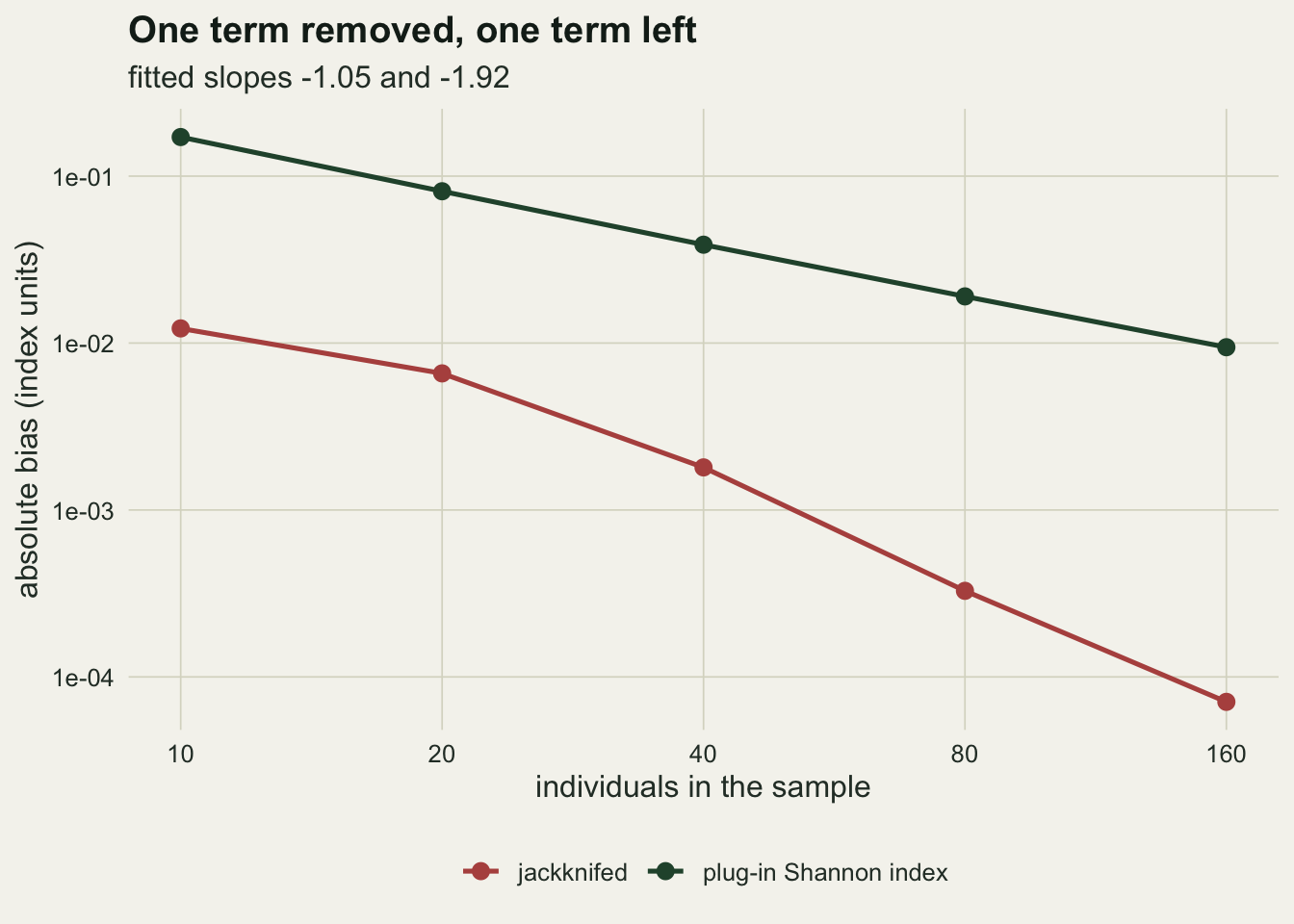
The plug-in slope is -1.05 and the jackknifed slope is -1.92. Over the upper three sample sizes alone the jackknifed slope is -2.33, which is past minus two rather than short of it. Multiplying the corrected bias by the square of the sample size leaves a quantity that still falls by a factor of 1.59 between 40 and 160 individuals, so terms beyond the one over n squared term are still adding to the corrected bias at these sizes and fading as the sample grows, and a slope fitted over a narrow window at the upper end reads steeper than the asymptotic one, while the fit over all five sizes reads shallower because the small sample end drags it. The corrected line is not parallel to the raw one, which is the point: the benefit of the correction is not a fixed factor but grows with sample size, and at the long plot’s effort it is a factor of 133.
The slope of the corrected line is a little shallower than minus two over the full range, and the reason is visible at the left edge. At the smallest sample size the rarest species is missing from a large share of samples, and an estimator computed from a sample in which a species never appears is not well described by a smooth expansion in one over n. The cancellation is asymptotic, and the small sample end is where it is weakest.
The jackknife variance of a median rests on one spacing
The same pseudo-values that correct the bias also supply a variance estimate, and this is where the method parts company with the bootstrap. Take the beetle masses and the median instead of the mean.
jk_med <- jack_parts(mass_g, median)
n_levels <- length(unique(round(jk_med$loo, 12)))
mass_sorted <- sort(mass_g)
half <- n_mass / 2
central_gap <- mass_sorted[half + 1] - mass_sorted[half]
med_formula <- (n_mass - 1) * central_gap^2 / 4
id_medvar <- abs(jk_med$var_jack - med_formula)
mean_pseudo_sd <- sd(jk_mean$pseudo)
med_pseudo_sd <- sd(jk_med$pseudo)
Deleting an observation below the median moves the median up to the next order statistic; deleting one above moves it down to the previous one. Nothing else can happen, so the 20 delete-one medians take exactly 2 distinct values, and the jackknife variance reduces to the sample size minus one, times the squared gap between the two central observations, divided by four. That closed form agrees with the general computation to 0.0e+00.
Everything else in the sample is discarded. The estimate rests on a single spacing between two adjacent order statistics, and a single spacing does not settle down as the sample grows: it shrinks in size but its relative variability does not fall. That is the mechanism of the failure, and it is visible before any simulation is run.
ord <- order(mass_g)
pseudo_long <- data.frame(
  rank_i = rep(seq_len(n_mass), 2),
  value = c(jk_mean$pseudo[ord], jk_med$pseudo[ord]),
  kind = rep(c("mean", "median"), each = n_mass))

ggplot(pseudo_long, aes(rank_i, value, colour = kind)) +
  geom_point(size = 2.6) +
  scale_colour_manual(values = c(te_forest, te_rust), name = NULL) +
  labs(x = "rank of the deleted observation", y = "pseudo-value (g)",
       title = "What each deletion is allowed to say",
       subtitle = sprintf("standard deviation of the pseudo-values: %.1f and %.1f g",
                          mean_pseudo_sd, med_pseudo_sd)) +
  theme_datasheet() +
  theme(legend.position = "bottom")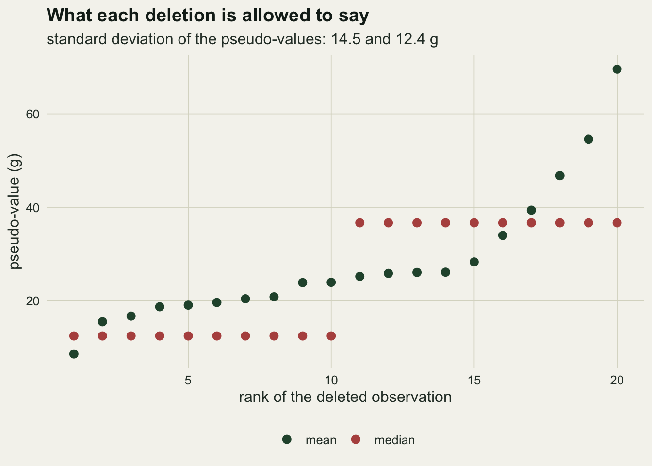
The median breaks the jackknife and not the bootstrap
The check is a sampling experiment: draw many samples of beetle masses, compute the true sampling variance of the median across them, and compare it with what the jackknife and the bootstrap report from each single sample. Replication was fixed before any of it ran: the claim is whether a ratio sits at one or near two, so the target was a Monte Carlo standard error on each ratio of about a tenth, and a pilot run fixed the count that reached it. That resolution answers the question the experiment was set for and no finer one, which matters for how the numbers below are read. Two hundred bootstrap resamples per sample are enough, because the inner resampling adds noise to the ratio but no bias to it.
fast_med <- function(dat) {
  m <- length(dat)
  sv <- sort(dat, partial = c(m / 2, m / 2 + 1))
  (sv[m / 2] + sv[m / 2 + 1]) / 2
}
med_jack_var <- function(dat) {
  m <- length(dat)
  sv <- sort(dat, partial = c(m / 2, m / 2 + 1))
  (m - 1) * (sv[m / 2 + 1] - sv[m / 2])^2 / 4
}
boot_var_med <- function(dat, n_boot) {
  m <- length(dat)
  var(vapply(seq_len(n_boot), function(b) fast_med(dat[sample.int(m, m, TRUE)]), 0))
}

n_rep <- 2000
n_boot <- 200
n_sweep <- c(20, 50, 200, 800)
keep <- vector("list", length(n_sweep))
sweep_tab <- NULL

for (k in seq_along(n_sweep)) {
  n_k <- n_sweep[k]
  set.seed(7000 + n_k)
  theta <- numeric(n_rep); v_j <- numeric(n_rep); v_b <- numeric(n_rep)
  for (r in seq_len(n_rep)) {
    dat <- rlnorm(n_k, log(28), 0.55)
    theta[r] <- fast_med(dat)
    v_j[r] <- med_jack_var(dat)
    v_b[r] <- boot_var_med(dat, n_boot)
  }
  v_true <- var(theta)
  keep[[k]] <- data.frame(n = n_k, jackknife = v_j / v_true, bootstrap = v_b / v_true)
  sweep_tab <- rbind(sweep_tab, data.frame(
    n = n_k, v_true = v_true,
    jack = mean(v_j) / v_true, jack_se = sd(v_j) / sqrt(n_rep) / v_true,
    boot = mean(v_b) / v_true, boot_se = sd(v_b) / sqrt(n_rep) / v_true))
}
mcse_max <- max(sweep_tab$jack_se)
jack_drop <- sweep_tab$jack[1] - sweep_tab$jack[4]
jack_drop_se <- sqrt(sweep_tab$jack_se[1]^2 + sweep_tab$jack_se[4]^2)
That is 2000 samples at each of four sizes. The jackknife variance estimate of the median averages about 2.2 times the true sampling variance at the smallest sample size and about 2.0 times it at the largest, and nowhere in that fortyfold increase in sample size does it come near one. The Monte Carlo standard error on each of those ratios is 0.11 at worst, which is far smaller than the distance between two and one and not small enough to resolve the drift within the sequence: the fall from the first ratio to the last is 0.20, with a standard error of 0.15 on it. The reading this experiment supports is that the ratio sits near two and is not heading for one, not a value for its third decimal or a slope across the four sizes. The bootstrap on the same samples returns 1.32, 1.14, 1.09 and 1.03, falling steadily towards one.
ratio_long <- rbind(
  data.frame(n = sweep_tab$n, ratio = sweep_tab$jack, se = sweep_tab$jack_se,
             method = "jackknife"),
  data.frame(n = sweep_tab$n, ratio = sweep_tab$boot, se = sweep_tab$boot_se,
             method = "bootstrap"))

ggplot(ratio_long, aes(n, ratio, colour = method)) +
  geom_hline(yintercept = 1, linetype = "dashed", colour = te_ink, linewidth = 0.6) +
  geom_line(linewidth = 0.9) +
  geom_errorbar(aes(ymin = ratio - se, ymax = ratio + se), width = 0.05,
                linewidth = 0.5) +
  geom_point(size = 2.6) +
  scale_x_log10(breaks = n_sweep) +
  scale_colour_manual(values = c(te_forest, te_rust), name = NULL) +
  labs(x = "sample size", y = "estimated variance / true variance",
       title = "One of them converges",
       subtitle = "dashed line: an honest variance estimate") +
  theme_datasheet() +
  theme(legend.position = "bottom")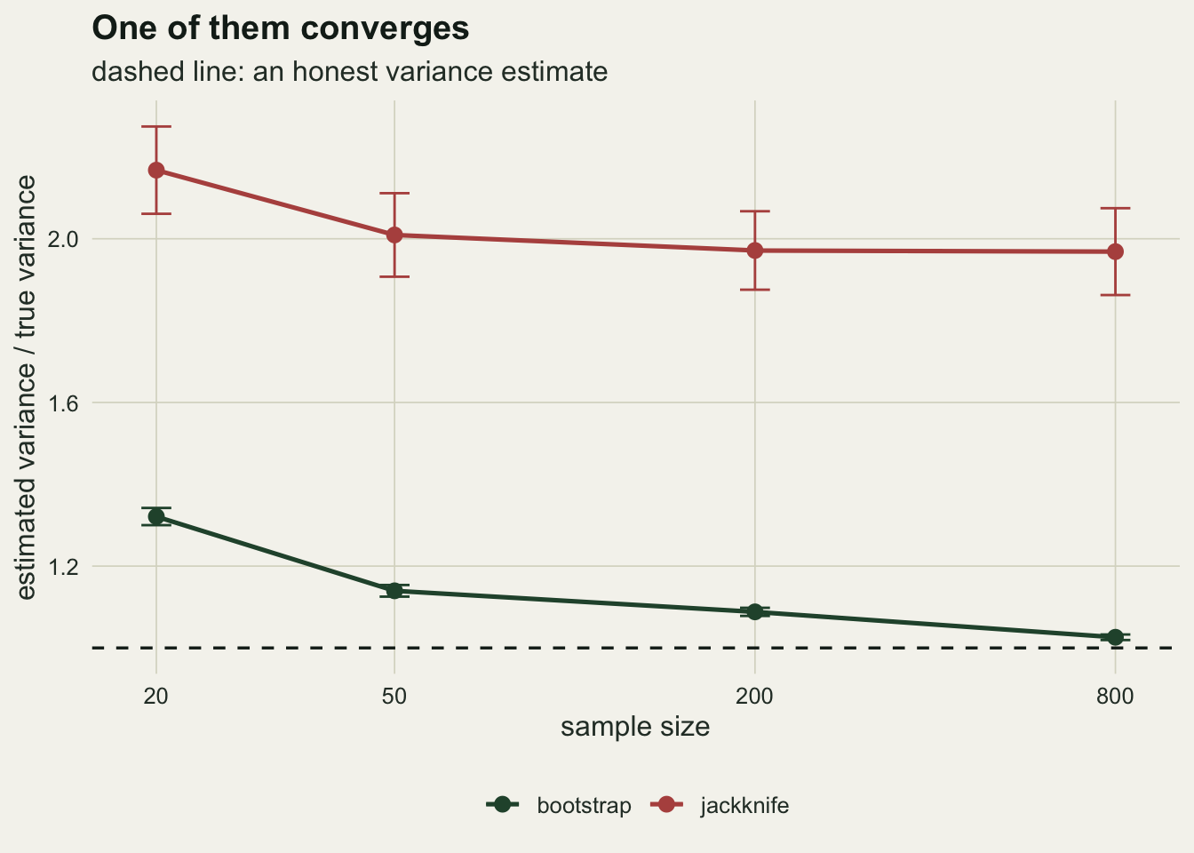
The direction is not the surprise. Efron and Stein proved that the delete-one variance estimate is biased upwards for a statistic symmetric in its arguments, so the jackknife errs high by construction and a ratio above one is what that result leads you to expect. The size is another matter, and a mean ratio of two would in any case be fixable: divide by two and move on. The deeper failure is that the jackknife estimate does not settle on any value at all.
spread_dat <- rbind(
  data.frame(n = keep[[1]]$n, ratio = keep[[1]]$jackknife, method = "jackknife"),
  data.frame(n = keep[[1]]$n, ratio = keep[[1]]$bootstrap, method = "bootstrap"),
  data.frame(n = keep[[4]]$n, ratio = keep[[4]]$jackknife, method = "jackknife"),
  data.frame(n = keep[[4]]$n, ratio = keep[[4]]$bootstrap, method = "bootstrap"))
spread_dat$panel <- factor(paste("n =", spread_dat$n),
                           levels = paste("n =", c(n_sweep[1], n_sweep[4])))
cv_small <- sd(keep[[1]]$jackknife) / mean(keep[[1]]$jackknife)
cv_large <- sd(keep[[4]]$jackknife) / mean(keep[[4]]$jackknife)
cv_boot_small <- sd(keep[[1]]$bootstrap) / mean(keep[[1]]$bootstrap)
cv_boot_large <- sd(keep[[4]]$bootstrap) / mean(keep[[4]]$bootstrap)
over_three <- 100 * mean(keep[[4]]$jackknife > 3)ggplot(spread_dat, aes(ratio, colour = method)) +
geom_density(linewidth = 0.9, adjust = 1.2) +
geom_vline(xintercept = 1, linetype = "dashed", colour = te_ink, linewidth = 0.5) +
coord_cartesian(xlim = c(0, 6)) +
facet_wrap(~ panel) +
scale_colour_manual(values = c(te_forest, te_rust), name = NULL) +
labs(x = "estimated variance / true variance", y = "density",
title = "The bootstrap concentrates, the jackknife does not",
subtitle = "same experiment, forty times the data on the right") +
theme_datasheet() +
theme(legend.position = "bottom")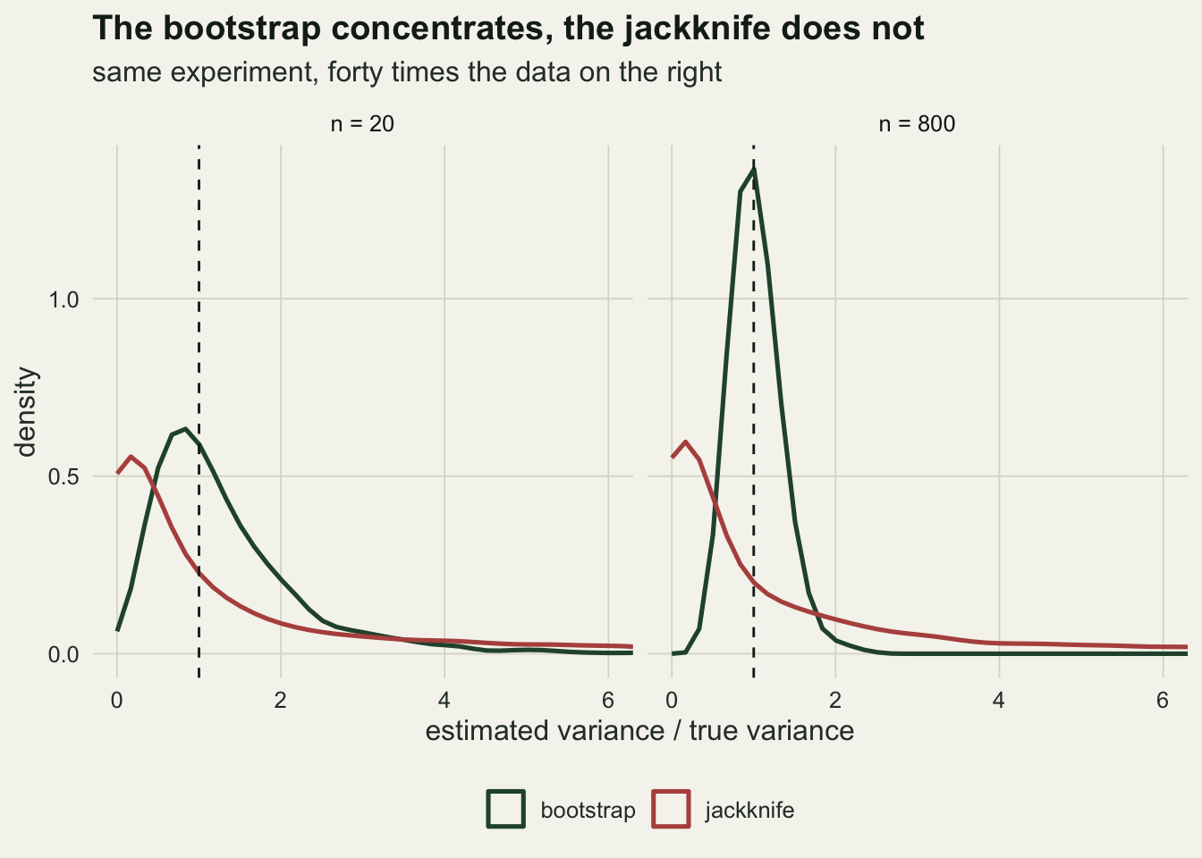
The bootstrap ratio tightens from a coefficient of variation of 0.71 to 0.29 as the sample grows fortyfold. The jackknife ratio goes from 2.20 to 2.41, which is not a fall but a slight rise, and at the largest sample size 17 per cent of samples still report a variance more than three times the true one. This is the inconsistency that Shao and Wu characterise: the jackknife variance estimator needs the statistic to be differentiable in a sense the median fails, and the failure does not weaken with sample size. Efron’s paper that introduced the bootstrap is titled as another look at the jackknife, and this is the gap it looked at.
The richness estimators are the same cancellation
The best known jackknife in ecology is not a variance estimate. The first order jackknife richness estimator adds to the observed species count a correction driven by the number of species found in exactly one sampling unit. It is usually presented as a formula. It is a delete-one calculation on the quadrats.
n_quad <- 12
n_pool <- 40
set.seed(5512)
det_p <- runif(n_pool, 0.02, 0.5)
occ_mat <- matrix(rbinom(n_pool * n_quad, 1, rep(det_p, times = n_quad)),
                  n_pool, n_quad)
occupancy <- rowSums(occ_mat)
s_obs <- sum(occupancy > 0)
q_one <- sum(occupancy == 1)

loo_rich <- vapply(seq_len(n_quad),
                   function(q) sum(rowSums(occ_mat[, -q, drop = FALSE]) > 0), 0)
jack_rich <- n_quad * s_obs - (n_quad - 1) * mean(loo_rich)
bo_formula <- s_obs + q_one * (n_quad - 1) / n_quad
id_rich <- abs(jack_rich - bo_formula)
Deleting a quadrat costs the survey exactly the species that were unique to it, so the average delete-one richness is the observed richness minus the number of uniques divided by the number of quadrats. Running that through the jackknife gives the Burnham and Overton estimator: with 12 quadrats, 32 species observed and 8 of them unique to a single quadrat, the delete-one computation returns 39.33 and the published formula returns the same to 3.6e-14. The true pool was 40 species, so on this survey the correction closes most of the gap and not all of it.
That is the honest reading of the richness estimators in the earlier post on this site. They are not detectors of unseen species. They are bias corrections on the observed count, they remove the term of order one over the number of sampling units, and what is left over is the reason they stay lower bounds. Zahl made the same argument for diversity indices, which is where the jackknifed Shannon index above comes from.
What to report
Say which quantity the jackknife was applied to and why. Correcting the bias of a plug-in diversity index is the use the method was designed for and it works; using it for the standard error of an awkward statistic is a different claim, and it needs the statistic to be smooth.
Report the uncorrected estimate next to the corrected one. The difference is a measurement of how far into the small sample regime the survey sits, and a correction that moves the index by a tenth of its value is telling you that the sample is thin, not that the problem is solved.
Give the sampling effort per unit alongside any index that is compared across units. A bias of order one over the sample size is an effort gradient in disguise, and equalising effort by rarefaction is often a better answer than correcting each value separately.
If the jackknife supplied a standard error, say what the statistic was. For a mean, a regression coefficient, a smooth function of moments, it is fine and it equals the familiar formula. For a median or an interior quantile, quote a bootstrap standard error instead, and say that you did. For an extreme, a sample minimum or maximum, a range, a parameter at the edge of its space, do not swap one resampling method for the other: the bootstrap is inconsistent there too, as checking a bootstrap shows for the maximum, and the honest routes are an exact result or a parametric model.
Honest limits
The exact enumeration covers four species and sample sizes up to 160. Real assemblages have long tails of rare species, the bias of a plug-in index is larger there, and the one over n expansion is a worse description because the probability of missing species entirely is higher. The direction of the result carries over; the numbers do not.
The bias correction is not free. The jackknifed Shannon index has a larger variance than the plug-in one, because the correction amplifies the sample-to-sample scatter along with the systematic part, and in a small sample the mean squared error can be worse after correcting. Nothing above measures that trade-off, and a post that recommended the correction without naming it would be selling half the picture.
The median experiment uses one distribution, a lognormal with a single central mode, and samples of even size. A distribution with a flat region or a gap near the median makes the jackknife worse, because the central spacing the estimate depends on becomes even more variable. An odd sample size changes the arithmetic slightly, giving three distinct delete-one values rather than two, and does not change the conclusion.
The bootstrap ratio above is still above one at the largest sample size, by 3 per cent. The bootstrap variance of a median is consistent, but its approach to the truth is slow, and reading the right hand end of that curve as an endorsement would be over-reading it. The claim is the contrast: one estimator is converging and the other is not.
The delete-one jackknife is not the only one. Deleting groups of observations, the delete-d jackknife, restores consistency for the median when the group size grows with the sample in the right way, and the same idea underlies the block jackknife for dependent data. That repair is real and it is not covered here; the point of this post is what the plain delete-one version does and does not do.
References
Quenouille MH 1956 Biometrika 43(3-4):353-360 (10.1093/biomet/43.3-4.353)
Miller RG 1974 Biometrika 61(1):1-15 (10.1093/biomet/61.1.1)
Efron B 1979 Annals of Statistics 7(1):1-26 (10.1214/aos/1176344552)
Efron B, Stein C 1981 Annals of Statistics 9(3):586-596 (10.1214/aos/1176345462)
Shao J, Wu CFJ 1989 Annals of Statistics 17(3):1176-1197 (10.1214/aos/1176347263)
Burnham KP, Overton WS 1978 Biometrika 65(3):625-633 (10.1093/biomet/65.3.625)
Zahl S 1977 Ecology 58(4):907-913 (10.2307/1936227)
Basharin GP 1959 Theory of Probability and Its Applications 4(3):333-336 (10.1137/1104033)