library(ggplot2)

te_pal <- list(forest = "#275139", green = "#2f8f63", sage = "#93a87f",
               clay = "#b5534e", gold = "#cda23f", line = "#dad9ca",
               ink = "#16241d")

theme_te <- function() {
  theme_minimal(base_size = 12) +
    theme(panel.grid.minor = element_blank(),
          panel.grid.major = element_line(colour = "#e7e6dc"),
          plot.background = element_rect(fill = "#f5f4ee", colour = NA),
          panel.background = element_rect(fill = "#f5f4ee", colour = NA),
          plot.title = element_text(face = "bold", colour = te_pal$ink),
          axis.title = element_text(colour = "#2c3a31"))
}Checking an effective size estimate
R
population genetics
model diagnostics
ecology tutorial
ggplot2
Four checks for an Ne estimate in R: which time window it covers, what sampling relatives does to it, how wide the interval is, and what linkage costs.
Corrected 14 October 2026: the temporal estimate in the first check subtracted the old sample’s sampling error as if that sample came from an unlimited population, though its individuals are a quarter of the population that breeds the next generation; it now applies the finite-population correction, which lowers the estimate slightly. The first check also said that five generations at the crashed size had barely dented gene diversity, and it now says they removed a modest share of it; the second check said that nothing in the genetic data flags the association that sampled families add, and it now says only that nothing in the linkage disequilibrium values does.
Corrected 1 October 2026: the current sample in the first check asked for fifty individuals from a population that by then held twenty, so it is the whole population, yet the temporal estimate still subtracted sampling error for a sample of fifty; it now treats that sample as a census, which lowers the estimate a little, and the interval section no longer calls it fifty individuals. The second check now says it simulates a new population rather than reusing the same one.
Corrected 30 September 2026: the jackknife section did not say that its symmetric interval ignores the skew of the estimate, and implied that its upper bound can run to infinity, which only an interval built on the drift signal and inverted can do; the linkage section called a linked-marker estimate a lower bound on Ne, and it now says the estimate is biased downward but can still land above the truth.
An effective size estimate is a single number attached to a large number of assumptions: a closed population, constant size, discrete generations, unlinked neutral markers, a random sample of unrelated individuals. Every one of those fails somewhere, and they do not all fail in the same direction.
Four checks, each a simulation with a known answer. The first is the one that resolves most published disagreements: two methods applied to the same population return different numbers because they measure different time windows, and both can be right.
The engine carries haplotypes at 40 biallelic loci with symmetric mutation, and takes a recombination rate so that loci can be made linked later.
gamete <- function(hap, par, n_loci, c_rec) {
  n_off <- length(par)
  if (c_rec >= 0.5) {
    which_hap <- matrix(sample(0:1, n_off * n_loci, replace = TRUE),
                        n_off, n_loci)
  } else {
    sw <- matrix(runif(n_off * n_loci) < c_rec, n_off, n_loci)
    sw[, 1] <- sample(c(TRUE, FALSE), n_off, replace = TRUE)
    which_hap <- t(apply(sw, 1, function(x) cumsum(x) %% 2))
  }
  rows <- 2 * par - 1 + which_hap
  matrix(hap[cbind(as.vector(rows), rep(seq_len(n_loci), each = n_off))],
         n_off, n_loci)
}

one_gen <- function(hap, n_next, u, c_rec) {
  n_now <- nrow(hap) / 2
  n_loci <- ncol(hap)
  h1 <- gamete(hap, sample(n_now, n_next, replace = TRUE), n_loci, c_rec)
  h2 <- gamete(hap, sample(n_now, n_next, replace = TRUE), n_loci, c_rec)
  out <- matrix(0L, 2 * n_next, n_loci)
  out[seq(1, 2 * n_next, by = 2), ] <- h1
  out[seq(2, 2 * n_next, by = 2), ] <- h2
  mut <- runif(length(out)) < u
  out[mut] <- 1L - out[mut]
  out
}

mean_r2 <- function(hap, maf_min = 0.05) {
  p <- colMeans(hap)
  keep <- pmin(p, 1 - p) >= maf_min
  cr <- suppressWarnings(cor(hap[, keep, drop = FALSE]))
  r2 <- cr[upper.tri(cr)]^2
  mean(r2[is.finite(r2)])
}

ld_ne <- function(hap_sample, n_perm = 5) {
  obs <- mean_r2(hap_sample)
  floor_r2 <- mean(replicate(n_perm, mean_r2(apply(hap_sample, 2, sample))))
  c(r2_obs = obs, r2_floor = floor_r2, ne = 1 / (3 * (obs - floor_r2)))
}

take_sample <- function(hap, n_take) {
  n_ind <- nrow(hap) / 2
  take <- sort(sample(n_ind, min(n_take, n_ind)))
  hap[as.vector(rbind(2 * take - 1, 2 * take)), , drop = FALSE]
}

fc_ne <- function(x, y, t_gap, s0, st) {
  keep <- (x + y) > 0 & (x + y) < 2
  fc <- mean((x[keep] - y[keep])^2 /
               ((x[keep] + y[keep]) / 2 - x[keep] * y[keep]))
  t_gap / (2 * (fc - 1 / (2 * s0) - 1 / (2 * st)))
}
Check 1: which window does the estimate cover?
Build a population with a known history: 800 generations at 200 individuals to reach mutation-drift equilibrium, a sample taken 20 generations ago, then 15 more generations at 200 and a crash to 20 for the last five. Now estimate Ne three ways from the data that history leaves behind.
set.seed(472)
n_loci <- 40
u <- 2.5e-3
n_old <- 200
theta <- 4 * n_old * u

hap <- matrix(rbinom(2 * n_old * n_loci, 1, 0.5), nrow = 2 * n_old)
for (g in seq_len(800)) hap <- one_gen(hap, n_old, u, 0.5)
p_burn <- colMeans(hap)
cat("heterozygosity after burn-in:", round(mean(2 * p_burn * (1 - p_burn)), 4),
    " two-allele equilibrium theta/(2 theta + 1):",
    round(theta / (2 * theta + 1), 4), "\n")
heterozygosity after burn-in: 0.368 two-allele equilibrium theta/(2 theta + 1): 0.4 old_sample <- take_sample(hap, 50)
x_old <- colMeans(old_sample)
for (g in seq_len(15)) hap <- one_gen(hap, n_old, u, 0.5)
for (g in seq_len(5)) hap <- one_gen(hap, 20, u, 0.5)
now_sample <- take_sample(hap, 50)
y_now <- colMeans(now_sample)
ld_now <- ld_ne(now_sample)
# the current sample is the whole surviving population, so it adds no sampling error;
# the old sample is 50 of the 200 individuals that then breed, so its term takes the
# finite-population correction 1/(2 * 50) - 1/(2 * 200)
ne_temporal <- fc_ne(x_old, y_now, 20, 1 / (1 / 50 - 1 / n_old), Inf)
het_now <- mean(2 * y_now * (1 - y_now))
ne_diversity <- het_now / (4 * u * (1 - 2 * het_now))
cat("linkage disequilibrium estimate:", round(ld_now[["ne"]], 1), "\n")linkage disequilibrium estimate: 14.6 cat("temporal estimate over 20 generations:", round(ne_temporal, 1),
" harmonic mean of the true path over that window:",
round(20 / (15 / 200 + 5 / 20), 1), "\n")temporal estimate over 20 generations: 68.1 harmonic mean of the true path over that window: 61.5 cat("equilibrium-diversity estimate:", round(ne_diversity, 1),
" heterozygosity now:", round(het_now, 4), "\n")equilibrium-diversity estimate: 90.9 heterozygosity now: 0.3225 Three numbers from one population: 14.6, 68.1 and 90.9. None of them is wrong.
The linkage disequilibrium estimate is 14.6 against a true current size of 20, because associations between unlinked loci are rebuilt every generation and forgotten within a few, so this estimate sees the recent past. The temporal estimate is 68.1, and the harmonic mean of the true sizes across its 20-generation window is 61.5, so it is reporting the average of the window rather than either end of it. The diversity-based estimate inverts the equilibrium relation between heterozygosity and 4Nu, and returns 90.9: still weighted towards the long history at 200, because gene diversity takes on the order of N generations to respond and five generations at 20 have removed only a modest share of it.
The check to run, then, is not “do my estimates agree” but “what window does each of them cover, and is that the window my question is about”. A population that has just crashed will show a small LD estimate and a large diversity-based estimate, and that discrepancy is the signal, not an error.
true_df <- data.frame(generation = -25:0,
                      N = ifelse(-25:0 >= -5, 20, 200))
est_df <- data.frame(
  method = c("linkage disequilibrium", "temporal, 20 generations",
             "equilibrium diversity"),
  ne = c(ld_now[["ne"]], ne_temporal, ne_diversity),
  from = c(-5, -20, -25), to = c(0, 0, 0))

ggplot() +
  geom_step(data = true_df, aes(generation, N), colour = te_pal$ink,
            linewidth = 0.9, direction = "hv") +
  geom_segment(data = est_df, aes(x = from, xend = to, y = ne, yend = ne,
                                  colour = method), linewidth = 1.4) +
  scale_y_log10(breaks = c(10, 20, 50, 100, 200)) +
  scale_colour_manual(values = c(`linkage disequilibrium` = te_pal$clay,
                                 `temporal, 20 generations` = te_pal$gold,
                                 `equilibrium diversity` = te_pal$green),
                      name = NULL) +
  labs(title = "Three estimates, three time windows, one population",
       subtitle = "black step: true census size; coloured: each estimate over its window",
       x = "generations before the present", y = "individuals (log scale)") +
  theme_te()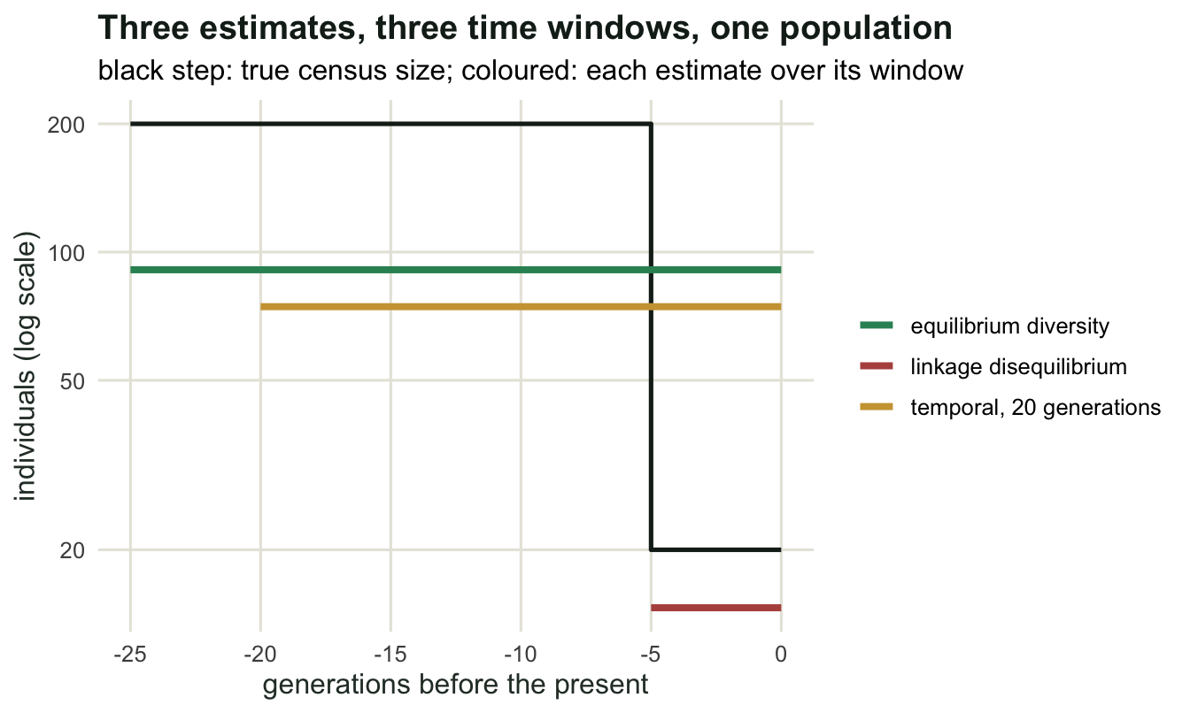
Check 2: are the sampled individuals related?
The linkage disequilibrium method assumes a random sample of unrelated individuals. Full siblings share parental haplotypes, which is a source of allelic association that has nothing to do with the size of the population, and field sampling produces siblings easily: a seed collection from few mother trees, a batch of juveniles from one pool, a family group at a den.
Simulate it directly. Take a new population of 200 and build samples of 50 individuals with different family structures, from 50 unrelated offspring to five families of ten.
set.seed(476)
pop <- matrix(rbinom(2 * 200 * n_loci, 1, 0.5), nrow = 2 * 200)
for (g in seq_len(60)) pop <- one_gen(pop, 200, u, 0.5)

make_sample <- function(pop, n_fam, per_fam) {
  n_ind <- nrow(pop) / 2
  kids <- NULL
  for (f in seq_len(n_fam)) {
    dad <- sample(n_ind, 1)
    mum <- sample(setdiff(seq_len(n_ind), dad), 1)
    h1 <- gamete(pop, rep(dad, per_fam), n_loci, 0.5)
    h2 <- gamete(pop, rep(mum, per_fam), n_loci, 0.5)
    for (k in seq_len(per_fam)) kids <- rbind(kids, h1[k, ], h2[k, ])
  }
  kids
}

fam_tab <- t(sapply(list(c(50, 1), c(25, 2), c(10, 5), c(5, 10)),
                    function(cfg) {
  est <- replicate(8, ld_ne(make_sample(pop, cfg[1], cfg[2]))[c("r2_obs", "ne")])
  c(families = cfg[1], per_family = cfg[2],
    r2_obs = mean(unlist(est[1, ])), Ne_median = median(unlist(est[2, ])))
}))
print(round(fam_tab, 4))
families per_family r2_obs Ne_median
[1,] 50 1 0.0115 327.5121
[2,] 25 2 0.0140 87.5783
[3,] 10 5 0.0211 30.9845
[4,] 5 10 0.0323 15.5411Fifty unrelated offspring give a median estimate of 327.5 for a population of 200, which is the familiar upward noise when the drift signal is small. Two siblings per family already pull it to 87.6. Five per family give 31.0, and ten per family give 15.5: a population of 200 looks like a population of 16, an error of more than tenfold, in the dangerous direction for a conservation decision.
The r^2 column shows why. It climbs from 0.0115 to 0.0323 as families get larger, and the estimator has no way to tell family-generated association from drift-generated association. Nothing in the r^2 values flags it either, which is why the check has to be done on the sampling design: relatedness screening before estimation, or one individual per family, or a method that models the family structure. That repair is written for a sample built out of families. Applied to a randomly sampled cohort it manufactures the opposite error, because the siblings a random sample contains are part of the signal the method reads, and purging siblings before estimating Ne measures how far the estimate moves when they are taken out.
fam_df <- as.data.frame(fam_tab)
fam_df$label <- sprintf("%d x %d", fam_df$families, fam_df$per_family)
fam_df$label <- factor(fam_df$label, levels = fam_df$label)

ggplot(fam_df, aes(label, Ne_median)) +
  geom_col(fill = te_pal$clay, colour = "white", width = 0.6) +
  geom_hline(yintercept = 200, linetype = "dashed", colour = te_pal$ink) +
  geom_text(aes(label = round(Ne_median, 0)), vjust = -0.4, size = 4,
            colour = "#2c3a31") +
  scale_y_continuous(expand = expansion(mult = c(0.05, 0.1))) +
  labs(title = "Siblings in the sample shrink the population",
       subtitle = "families x offspring per family, 50 individuals in total, true size 200",
       x = "sample structure", y = "median estimated Ne") +
  theme_te()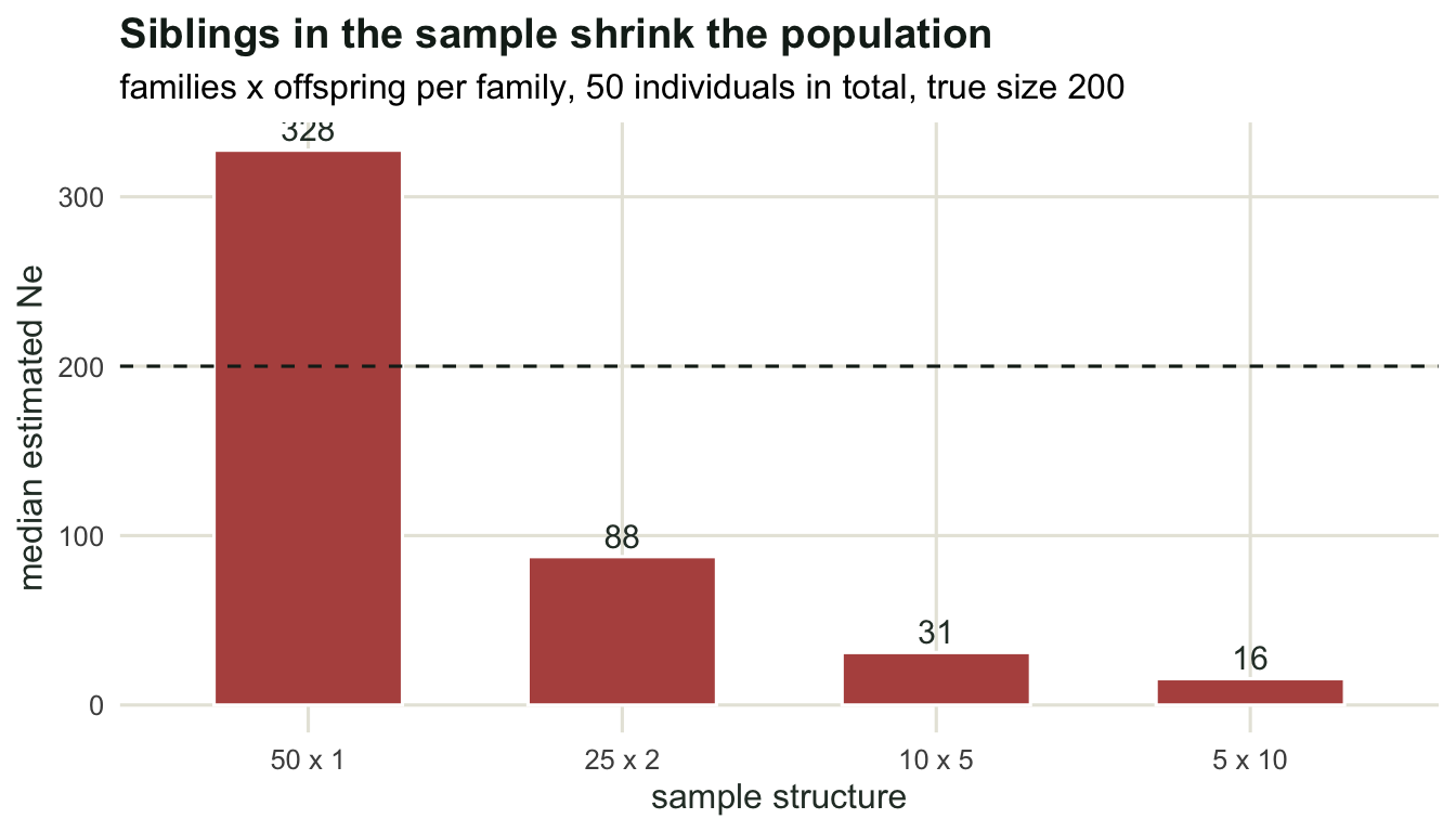
Check 3: how wide is the interval?
A point estimate of Ne is close to useless without an interval, and the interval is easy to get by leaving out one locus at a time.
jack_ld <- function(hap_sample) {
  n_l <- ncol(hap_sample)
  full <- ld_ne(hap_sample)[["ne"]]
  drop1 <- sapply(seq_len(n_l), function(j) ld_ne(hap_sample[, -j])[["ne"]])
  pseudo <- n_l * full - (n_l - 1) * drop1
  se <- sqrt(var(pseudo) / n_l)
  c(ne = full, se = se, lower = full - 1.96 * se, upper = full + 1.96 * se)
}

set.seed(474)
print(round(jack_ld(now_sample), 1))
ne se lower upper
14.5 4.9 4.9 24.1 The estimate is 14.5 with a jackknife standard error of 4.9, so the interval runs from 4.9 to 24.1 and on this sample contains the true current size of 20. It reads 14.5 here rather than the 14.6 above because the permutation floor inside ld_ne is redrawn under this chunk’s seed. That interval is the honest output here, though a rough one: Ne is the reciprocal of a small drift signal, so its sampling distribution is skewed, and published methods build the interval on the drift signal and then invert it. With 40 loci and a sample that is the whole of the current population, this analysis distinguishes “very small” from “not very small” and nothing finer. Report it that way, and note that on an inverted interval the upper bound often runs to infinity, which is the correct statement that the data cannot rule out a large population.
Check 4: are the loci actually unlinked?
The 1/(3Ne) expectation assumes free recombination between the markers. Physical linkage adds association that persists across generations, so linked loci inflate r^2 and deflate Ne. Repeat the estimate on populations of 100 with three recombination rates.
set.seed(475)
link_tab <- t(sapply(c(0.5, 0.2, 0.05), function(c_rec) {
  est <- replicate(8, {
    h <- matrix(rbinom(2 * 100 * n_loci, 1, 0.5), nrow = 2 * 100)
    for (g in seq_len(40)) h <- one_gen(h, 100, u, c_rec)
    ld_ne(take_sample(h, 50))[c("r2_obs", "ne")]
  })
  c(recombination = c_rec, r2_obs = mean(unlist(est[1, ])),
    Ne_median = median(unlist(est[2, ])))
}))
print(round(link_tab, 4))
recombination r2_obs Ne_median
[1,] 0.50 0.0131 115.3679
[2,] 0.20 0.0141 82.1995
[3,] 0.05 0.0174 42.6147At free recombination the estimate is 115.4 for a true size of 100. At a recombination rate of 0.2 between neighbouring markers it drops to 82.2, and at 0.05 to 42.6, with r^2 rising from 0.0131 to 0.0174. Dense marker panels from reduced-representation sequencing are full of linked pairs, and the bias is systematic and downward. Published implementations handle this by filtering pairs by map distance or by fitting the dependence of r^2 on recombination rate; if neither is possible, the estimate is biased downward and tends to understate Ne, although sampling noise alone can still put a single estimate above the true value.
The honest limit
Two things do not follow from any of this.
First, Ne is defined relative to a model, and the model matters more than the estimator. In a population with overlapping generations, an Ne estimated per generation and an Ne estimated per year differ by the generation length, and the simulations here have discrete generations by construction, so they cannot show that error. The same applies to selection: markers linked to anything under selection have their own coalescent history, and no single-sample diagnostic separates that from demography.
Second, an Ne estimate does not license a genetic-viability conclusion on its own. The thresholds in the literature refer to processes: inbreeding accumulating at a rate of 1/(2Ne) per generation, and mutation replenishing quantitative variation as fast as drift removes it. Both are statements about rates in an idealised population, and neither is a claim that a specific population with a specific Ne will or will not persist. The number is an input to that argument, not the argument.
Where to go next
That closes the effective-size cluster: what Ne means, two ways to estimate it, what a bottleneck does to the markers, and the checks. The natural next step is the other view of the same process, where instead of following allele frequencies forward you follow ancestries backward: the coalescent, where the shape of a gene tree carries the same demographic information in a different currency.
References
Waples RS 1989 Genetics 121(2):379-391 (10.1093/genetics/121.2.379)
Waples RS, Do C 2010 Evolutionary Applications 3(3):244-262 (10.1111/j.1752-4571.2009.00104.x)
Waples RS, England PR 2011 Genetics 189(2):633-644 (10.1534/genetics.111.132233)
Wang J, Santiago E, Caballero A 2016 Heredity 117(4):193-206 (10.1038/hdy.2016.43)