library(ggplot2)
library(patchwork)

te_paper  <- "#f5f4ee"
te_ink    <- "#16241d"
te_body   <- "#2c3a31"
te_forest <- "#275139"
te_rust   <- "#b5534e"
te_gold   <- "#c9b458"
te_line   <- "#dad9ca"

theme_datasheet <- function() {
  theme_minimal(base_size = 12) +
    theme(plot.background  = element_rect(fill = te_paper, colour = NA),
          panel.background = element_rect(fill = te_paper, colour = NA),
          panel.grid.major = element_line(colour = te_line, linewidth = 0.3),
          panel.grid.minor = element_blank(),
          text             = element_text(colour = te_body),
          plot.title       = element_text(colour = te_ink, face = "bold"),
          plot.subtitle    = element_text(colour = te_body),
          axis.text        = element_text(colour = te_body))
}Temporal Ne with overlapping generations: plan II bias
R
population genetics
effective population size
simulation
ecology tutorial
Temporal Ne from cohorts a few years apart can be negative. An R simulation shows the Waples 1989 plan II term sets the bias, and when adding it back works.
Suppose a small, closed population of a long lived bird has been monitored since 2012, and every chick is ringed and blood sampled in the nest. Assume, as the simplest model below does, that the chicks of a year are exactly the birds that will later replace the adults that died, so a sample of a few dozen is a large share of its cohort. Ten years later somebody genotypes the 2012 and the 2016 chicks on a SNP panel and estimates the effective population size from the change in allele frequencies between them. Four years is under two generations for a bird that breeds for many seasons, and the estimate that comes back is negative. The second attempt, 2012 against 2020, gives a number well above the effective size the population really has. A river population of brown trout, with fin clips from a few dozen young of the year out of thousands and a few females producing most of each cohort, can make the opposite error from the same kind of archive, and the last section shows why.
The temporal method on this site assumes none of that. The post on estimating Ne from genetic data builds the standardised variance of Nei and Tajima, subtracts one over twice the sample size for each sample, and converts the remaining drift into an effective size, all in a population with discrete generations whose samples are binomial draws from an allele frequency. Its checking companion, checking an effective size estimate, says out loud in its honest limit that its simulations have discrete generations by construction and so cannot show the error that comes with overlapping ones. The post on effective population size separates inbreeding and variance effective sizes and the time windows they describe. This post takes the gap those posts name and measures it: an age structured population, samples of newborns and of adults a given number of years apart, and the estimator applied the way it usually is.
The obvious story is that consecutive cohorts share parents, so their allele frequencies are too similar and the drift between them is underestimated. The simulation below agrees with the symptom, but the offset it measures is a term Waples 1989 already wrote down: the correction for his sampling plan II, in which individuals are sampled before they reproduce, from a population of known census size. The shared parent carry over is one part of that term, not a separate effect. What this post adds is the measurement in an age structured population: the standard choice between Waples’s plan I and plan II accounts for the bias of both newborn and adult samples in the simplest life history, and where a newborn sample sits between the two plans depends on how much of the sampled cohort goes on to breed, which also sets what share of the cohort a sample of fixed size is.
An age structured population with a known Ne
Every year a fixed number of adults breed at random: each newborn gets two parents drawn with replacement from the adult pool, with equal chances for every adult whatever its age. Then a fixed share of the adults dies at random, and the survivors are joined by as many recruits as there were deaths, so the pool stays at the same size. Survival does not depend on age, so the ages of adults are geometric and the mean age of a parent is one over one minus survival. A survival of zero is the control: every adult breeds once and dies, and generations are discrete.
All replicate populations of one life history live in one genotype matrix, one block of rows per replicate, and deaths overwrite rows in place. That keeps every year to a few matrix operations instead of a loop over replicates. In a sampling year the newborn cohort is larger than the recruits when juvenile survival is below one, and only the individuals that are either sampled or recruited are generated; the overlap between the two sets is drawn from the hypergeometric distribution, which is exact because newborns of one year are exchangeable.
n_ad    <- 250          # adults, constant every year
n_loci  <- 300          # unlinked biallelic loci
n_samp  <- 50           # individuals per genetic sample
n_rep   <- 48           # replicate populations per life history
n_year  <- 100          # years simulated
y_first <- 20           # year of the first sample
gaps    <- c(1, 2, 4, 8, 16)
surv_set <- c(0, 0.3, 0.6, 0.8)

sim_pop <- function(s, juv = 1, shape = Inf, ns = n_samp) {
  n_tot <- n_rep * n_ad
  p_start <- runif(n_rep * n_loci, 0.2, 0.8)
  geno <- matrix(rbinom(n_tot * n_loci, 2, rep(p_start, each = n_ad)), n_tot, n_loci)
  age  <- rgeom(n_tot, 1 - s) + 1
  blk  <- rep(seq_len(n_rep), each = n_ad)
  offs <- (seq_len(n_rep) - 1) * n_ad
  n_rec  <- round(n_ad * (1 - s))
  n_born <- round(n_rec / juv)
  samp_years <- c(y_first, y_first + gaps)
  het <- matrix(0, n_year, n_rep)
  age_sum <- 0; age_n <- 0
  newborn <- list(); adult <- list()
  kids_of <- function(n_k) {
    if (is.infinite(shape)) {
      idx <- sample.int(n_ad, 2 * n_k * n_rep, TRUE) + rep(offs, each = 2 * n_k)
    } else {
      idx <- unlist(lapply(offs, function(o)
        sample.int(n_ad, 2 * n_k, TRUE, prob = rgamma(n_ad, shape)) + o))
    }
    gam <- floor(geno[idx, , drop = FALSE] / 2 + runif(length(idx) * n_loci))
    odd <- seq(1, length(idx), 2)
    list(g = gam[odd, , drop = FALSE] + gam[odd + 1, , drop = FALSE], pa = age[idx])
  }
  by_rep <- function(g, m) rowsum(g, rep(seq_len(n_rep), each = m)) / (2 * m)
  for (y in seq_len(n_year)) {
    if (y %in% samp_years) {
      ai <- unlist(lapply(offs, function(o) sample.int(n_ad, ns) + o))
      adult[[as.character(y)]] <- by_rep(geno[ai, ], ns)
      ov  <- rhyper(n_rep, n_rec, n_born - n_rec, ns)
      n_k <- max(n_rec + ns - ov)
      kids <- kids_of(n_k)
      bs  <- (seq_len(n_rep) - 1) * n_k
      rec <- unlist(lapply(bs, function(b) b + seq_len(n_rec)))
      smp <- unlist(lapply(seq_len(n_rep), function(i)
        bs[i] + c(seq_len(ov[i]), n_rec + seq_len(ns - ov[i]))))
      newborn[[as.character(y)]] <- by_rep(kids$g[smp, ], ns)
      kids$g <- kids$g[rec, , drop = FALSE]
    } else {
      kids <- kids_of(n_rec)
    }
    age_sum <- age_sum + sum(kids$pa); age_n <- age_n + length(kids$pa)
    dead <- unlist(lapply(offs, function(o) sample.int(n_ad, n_rec) + o))
    geno[dead, ] <- kids$g
    age <- age + 1; age[dead] <- 1
    pf <- rowsum(geno, blk) / (2 * n_ad)
    het[y, ] <- rowMeans(2 * pf * (1 - pf))
  }
  list(s = s, juv = juv, shape = shape, het = het, gen_time = age_sum / age_n,
       newborn = newborn, adult = adult, n_born = n_born, n_rec = n_rec, ns = ns)
}

fc_nt <- function(x, y) {
  m <- (x + y) / 2
  v <- (x - y)^2 / (m - x * y)
  v[!(m > 0 & m < 1)] <- NA
  rowMeans(v, na.rm = TRUE)
}
The truth is the inbreeding effective size per generation. Expected heterozygosity of the adult pool decays by a factor of one minus one over twice the effective size per generation, so the slope of its logarithm against years, pooled over replicates, gives the effective size per year, and dividing by the generation time gives it per generation. The generation time is the mean age of the parents actually drawn in the simulation, not the formula. Both then get an analytic check. For random breeding with Poisson family sizes, the variance in lifetime family size of an individual entering the pool is two plus four times survival, and Hill 1979 showed that the effective size of such a population is the one of a discrete generation population with the same number of entrants per generation and the same variance, which here works out as the adult number divided by one plus survival.
summarise_run <- function(r) {
  yrs <- 10:n_year
  slope_yr <- unname(coef(lm(log(rowMeans(r$het[yrs, ])) ~ yrs))[2])
  ne_true <- -1 / (2 * slope_yr) / r$gen_time
  est <- do.call(rbind, lapply(gaps, function(g) {
    f_new <- fc_nt(r$newborn[[as.character(y_first)]], r$newborn[[as.character(y_first + g)]]) - 1 / r$ns
    f_ad  <- fc_nt(r$adult[[as.character(y_first)]],   r$adult[[as.character(y_first + g)]])   - 1 / r$ns
    data.frame(s = r$s, gap = g, rep = seq_len(n_rep), f_new = f_new, f_ad = f_ad)
  }))
  est$gen <- est$gap / r$gen_time
  est$ne_new     <- est$gen / (2 * est$f_new)
  est$ne_ad      <- est$gen / (2 * est$f_ad)
  est$ne_new_cen <- est$gen / (2 * (est$f_new + 1 / n_ad))
  est$ne_ad_cen  <- est$gen / (2 * (est$f_ad + 1 / n_ad))
  list(gen_time = r$gen_time, ne_true = ne_true, est = est)
}
set.seed(3107)
runs <- lapply(surv_set, sim_pop)
sums <- lapply(runs, summarise_run)
tab_truth <- data.frame(s = surv_set,
                        gen_sim = vapply(sums, `[[`, 0, "gen_time"),
                        gen_an  = 1 / (1 - surv_set),
                        ne_sim  = vapply(sums, `[[`, 0, "ne_true"),
                        ne_hill = n_ad / (1 + surv_set))
tv <- function(s, col) tab_truth[[col]][tab_truth$s == s]
ne_gap_max <- max(abs(tab_truth$ne_sim / tab_truth$ne_hill - 1))
tab_truth
s gen_sim gen_an ne_sim ne_hill
1 0.0 1.000000 1.000000 246.4511 250.0000
2 0.3 1.429243 1.428571 195.5493 192.3077
3 0.6 2.499519 2.500000 160.0572 156.2500
4 0.8 4.981308 5.000000 139.6106 138.8889With 250 adults the effective size per generation from heterozygosity decay is 246.5 for discrete generations, 195.5, 160.1 and 139.6 at survivals of 0.3, 0.6 and 0.8, against Hill values of 250.0, 192.3, 156.2 and 138.9; the largest relative gap is 2.4 per cent. The simulated generation time at a survival of 0.8 is 4.981 years against a formula value of 5.0. These are the numbers every estimate below is divided by.
The standard estimator on newborn cohorts
The estimator is the one from the neighbour post: the Nei and Tajima standardised variance over 300 loci, minus one over twice the sample size for each of two samples of 50 newborns, and the interval in years divided by the simulated generation time to get generations. The first sample is taken in year 20, the second one to sixteen years later, in 48 replicate populations per life history. Because estimates can be negative, the summaries are the median and the share of negative estimates, not a mean or a harmonic mean over replicates.
est_all <- do.call(rbind, lapply(sums, function(x) {
  e <- x$est; e$ne_true <- x$ne_true; e
}))
tab_main <- do.call(rbind, lapply(split(est_all, list(est_all$s, est_all$gap)), function(e)
  data.frame(s = e$s[1], gap = e$gap[1], gen = e$gen[1], ne_true = e$ne_true[1],
             med_new = median(e$ne_new), neg_new = mean(e$f_new < 0),
             med_ad = median(e$ne_ad), neg_ad = mean(e$f_ad < 0),
             med_new_cen = median(e$ne_new_cen), neg_new_cen = mean(e$f_new + 1 / n_ad < 0),
             med_ad_cen = median(e$ne_ad_cen), neg_ad_cen = mean(e$f_ad + 1 / n_ad < 0),
             mean_f_new = mean(e$f_new), se_f_new = sd(e$f_new) / sqrt(nrow(e)),
             mean_f_ad = mean(e$f_ad), se_f_ad = sd(e$f_ad) / sqrt(nrow(e)))))
tab_main <- tab_main[order(tab_main$s, tab_main$gap), ]
cell <- function(s, g, col) tab_main[[col]][tab_main$s == s & tab_main$gap == g]
ratio <- function(s, g, col) cell(s, g, col) / cell(s, g, "ne_true")
mcse_share <- sqrt(0.25 / n_rep)
samp_share <- pmin(1, n_samp / round(n_ad * (1 - surv_set)))
round(tab_main[, c("s", "gap", "med_new", "neg_new", "med_ad_cen")], 2)
s gap med_new neg_new med_ad_cen
0.1 0.0 1 -171.61 0.85 271.37
0.2 0.0 2 -349.54 0.56 313.18
0.4 0.0 4 464.03 0.02 267.70
0.8 0.0 8 351.79 0.00 258.37
0.16 0.0 16 299.67 0.00 269.51
0.3.1 0.3 1 -125.69 0.90 136.34
0.3.2 0.3 2 -282.17 0.65 207.07
0.3.4 0.3 4 421.88 0.10 193.64
0.3.8 0.3 8 272.92 0.00 195.93
0.3.16 0.3 16 237.69 0.00 203.14
0.6.1 0.6 1 -70.53 0.94 88.31
0.6.2 0.6 2 -167.27 0.77 127.07
0.6.4 0.6 4 318.50 0.29 165.73
0.6.8 0.6 8 277.26 0.00 158.23
0.6.16 0.6 16 198.81 0.00 164.19
0.8.1 0.8 1 -33.82 0.98 17.96
0.8.2 0.8 2 -75.58 0.94 60.65
0.8.4 0.8 4 -146.30 0.67 117.53
0.8.8 0.8 8 233.96 0.17 150.52
0.8.16 0.8 16 221.43 0.00 143.64At a survival of 0.6, a generation time of 2.5 years and a true effective size of 160, newborn cohorts one year apart give a negative estimate in 94 per cent of replicates, and two years apart in 77 per cent. Four years apart the median is 318, 2.0 times the truth, with 29 per cent still negative; eight years apart it is 1.7 times and sixteen years apart 1.2 times the truth. At a survival of 0.8 the negative share is still 67 per cent at four years. The Monte Carlo standard error of any of these shares is at most 7.2 percentage points. Keep the size of the cohort in mind: every newborn recruits in this life history, so a cohort has only as many members as adults died, and the sample of 50 newborns is 20 per cent of its cohort for discrete generations, 29 per cent at a survival of 0.3, 50 per cent at 0.6 and the whole cohort at 0.8.
So far this is the expected picture, and the pattern the bird archive ran into. The awkward row is the control. With discrete generations, where no two cohorts share a parent, the estimate one generation apart is negative in 85 per cent of replicates and four generations apart the median is 1.9 times the truth.
surv_cols <- c("0" = te_ink, "0.3" = te_gold, "0.6" = te_forest, "0.8" = te_rust)
tab_main$surv <- factor(tab_main$s, levels = surv_set)
p_med <- ggplot(tab_main, aes(gap, med_new / ne_true, colour = surv)) +
  geom_hline(yintercept = 1, linetype = "dashed", colour = te_body) +
  geom_hline(yintercept = 0, colour = te_line) +
  geom_line(linewidth = 0.8) + geom_point(size = 2) +
  scale_x_log10(breaks = gaps) +
  scale_colour_manual(values = surv_cols, name = "adult survival") +
  labs(x = "years between samples", y = "median estimate / true Ne",
       title = "Median estimate") +
  theme_datasheet() + theme(legend.position = "bottom")
p_neg <- ggplot(tab_main, aes(gap, neg_new, colour = surv)) +
  geom_line(linewidth = 0.8) + geom_point(size = 2) +
  scale_x_log10(breaks = gaps) +
  scale_y_continuous(limits = c(0, 1)) +
  scale_colour_manual(values = surv_cols, name = "adult survival") +
  labs(x = "years between samples", y = "share of negative estimates",
       title = "Negative estimates") +
  theme_datasheet() + theme(legend.position = "bottom")
(p_med | p_neg) + plot_layout(guides = "collect") +
  plot_annotation(theme = theme_datasheet() + theme(legend.position = "bottom"))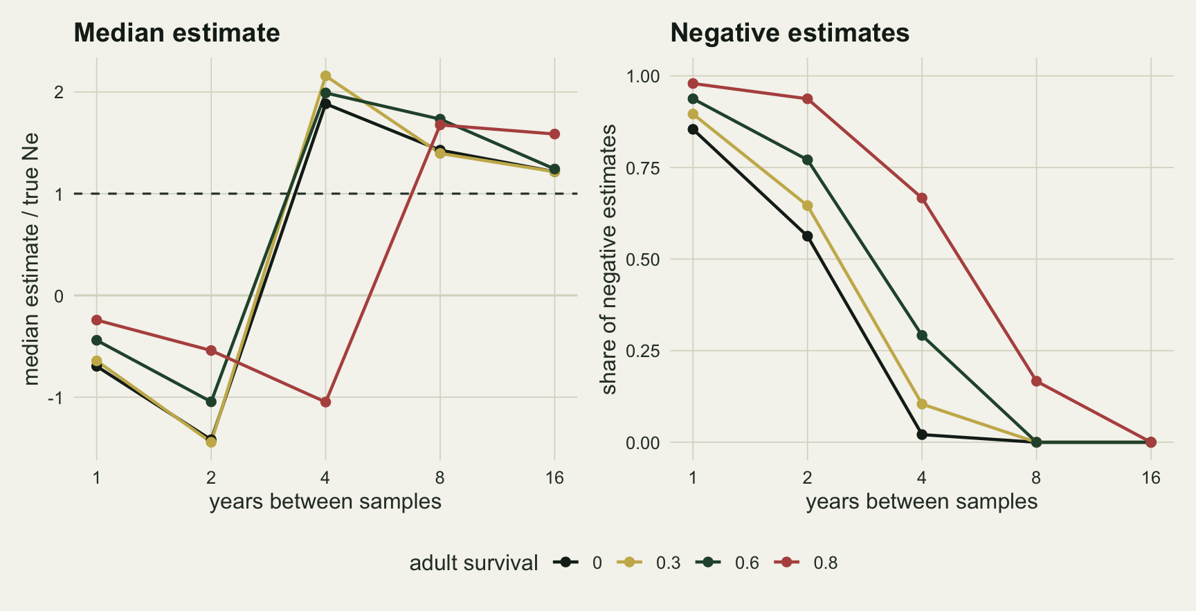
The bias is the plan II sampling term
Waples 1989 separates two ways of sampling. Under plan I, individuals are sampled after reproduction or with replacement, so the sample is independent of the genes passed to the next generation. Under plan II, individuals are sampled before reproduction and without replacement from a population of census size N, so the sampled individuals are among the parents of what follows; the usual sampling correction then removes too much, and his estimator adds one over N back: Ne = t / (2 [F - 1 / (2 S0) - 1 / (2 St) + 1 / N]), with S0 and St the two sample sizes. The question is which plan a newborn sample in an age structured population belongs to.
Write the frequency of an allele in the adult pool in year y as q, and the frequency among that year’s newborns as q plus a deviation e. With Poisson families and no juvenile mortality the deviation is binomial sampling of twice as many genes as there are recruits, so its variance is p(1 - p) over twice the number of recruits. Each year the pool keeps a random share s of its adults and takes in the recruits with weight 1 - s, so the recruits’ deviation e stays in the pool for good. Following the difference between a newborn sample in year y and one t years later through that recursion gives, after the usual sampling term is subtracted, an expected standardised variance of
t / (2 Ne T) - 1 / N
where N is the number of adults. The first term is the drift the estimator is meant to see. The second is negative, does not grow with the interval, and is the plan II term of Waples 1989. Two pieces make it up. The usual sampling term treats each newborn sample as a draw from an infinitely large cohort, but the cohort is finite, so the noise actually present in the samples is smaller than the amount removed. The cohort’s own deviation e would give that back, except that a share 1 - s of it passes into the pool that breeds the second cohort and cancels in the difference; this carry over is where shared parents enter, and at a survival of zero it is the whole deviation, because the first cohort is the parent pool of the next. What is left is minus 1 - s over the number of recruits, which is minus one over the number of adults when recruits replace deaths one for one, whatever the survival. A sample of adults drawn without replacement from the pool is a plan II sample in Waples’s own sense and gets the same term. A sample of newborns lands on the same one over N whatever the survival, as long as the whole cohort recruits: it is then drawn from individuals who will all breed, which makes it a plan II sample in all but name, with the shared parent carry over as one part of the term rather than a rival explanation.
The formula is a claim, so the chunk checks it against the simulated mean.
tab_main$pred_f <- tab_main$gen / (2 * tab_main$ne_true) - 1 / n_ad
tab_main$drift_f <- tab_main$gen / (2 * tab_main$ne_true)
z_new <- (tab_main$mean_f_new - tab_main$pred_f) / tab_main$se_f_new
z_ad  <- (tab_main$mean_f_ad  - tab_main$pred_f) / tab_main$se_f_ad
z_max <- max(abs(c(z_new, z_ad)))
z_med <- median(abs(c(z_new, z_ad)))
z_all <- c(z_new, z_ad); s_all <- rep(tab_main$s, 2); g_all <- rep(tab_main$gap, 2)
big <- abs(z_all) >= 3
n_big <- sum(big)
stopifnot(all(z_all[big] < 0), all(s_all[big] == 0), all(g_all[big] >= 4))
dev_all <- c(tab_main$mean_f_new, tab_main$mean_f_ad) - rep(tab_main$pred_f, 2)
short_max <- max(-dev_all[big] / rep(tab_main$drift_f, 2)[big])
crit_gen <- 2 / (1 + surv_set)
crit_yr  <- crit_gen * tab_truth$gen_sim
Across the four life histories and five intervals, the simulated mean of the corrected variance sits within 3.5 Monte Carlo standard errors of the prediction, for newborn samples and adult samples alike, and half of the cells are within 0.6 standard errors. All 3 deviations of three standard errors or more are negative and belong to the discrete generation control at intervals of four generations or longer, where the observed variance falls short of the prediction by at most 11 per cent of the drift term. The prediction uses a simulated true effective size that carries its own error (the control came out 1.4 per cent below its Hill value), and it ignores the loss of heterozygosity during the interval and the small sample bias of the standardised variance; those are the likely sources, and the post does not separate them. None of them touches the offset, which dominates at the short intervals where the estimates go negative. The offset itself, which is what matters at short intervals, is where the prediction puts it. Setting the prediction to zero gives the interval at which the estimate is expected to change sign: 2.00 generations for discrete generations and 1.11 generations, or 5.5 years, at a survival of 0.8. Measured in generations, overlapping generations shorten the danger zone a little. Measured in years, which is how freezers are organised, they lengthen it.
tab_main$surv_lab <- factor(paste("survival", tab_main$s), levels = paste("survival", surv_set))
ggplot(tab_main, aes(gen)) +
  geom_hline(yintercept = 0, colour = te_line, linewidth = 0.6) +
  geom_line(aes(y = drift_f), linetype = "dashed", colour = te_body) +
  geom_line(aes(y = pred_f), colour = te_forest, linewidth = 0.9) +
  geom_errorbar(aes(ymin = mean_f_new - 2 * se_f_new, ymax = mean_f_new + 2 * se_f_new),
                width = 0, colour = te_rust) +
  geom_point(aes(y = mean_f_new), colour = te_rust, size = 2) +
  facet_wrap(~ surv_lab, nrow = 1, scales = "free_x") +
  labs(x = "generations between samples", y = "mean corrected Fc") +
  theme_datasheet()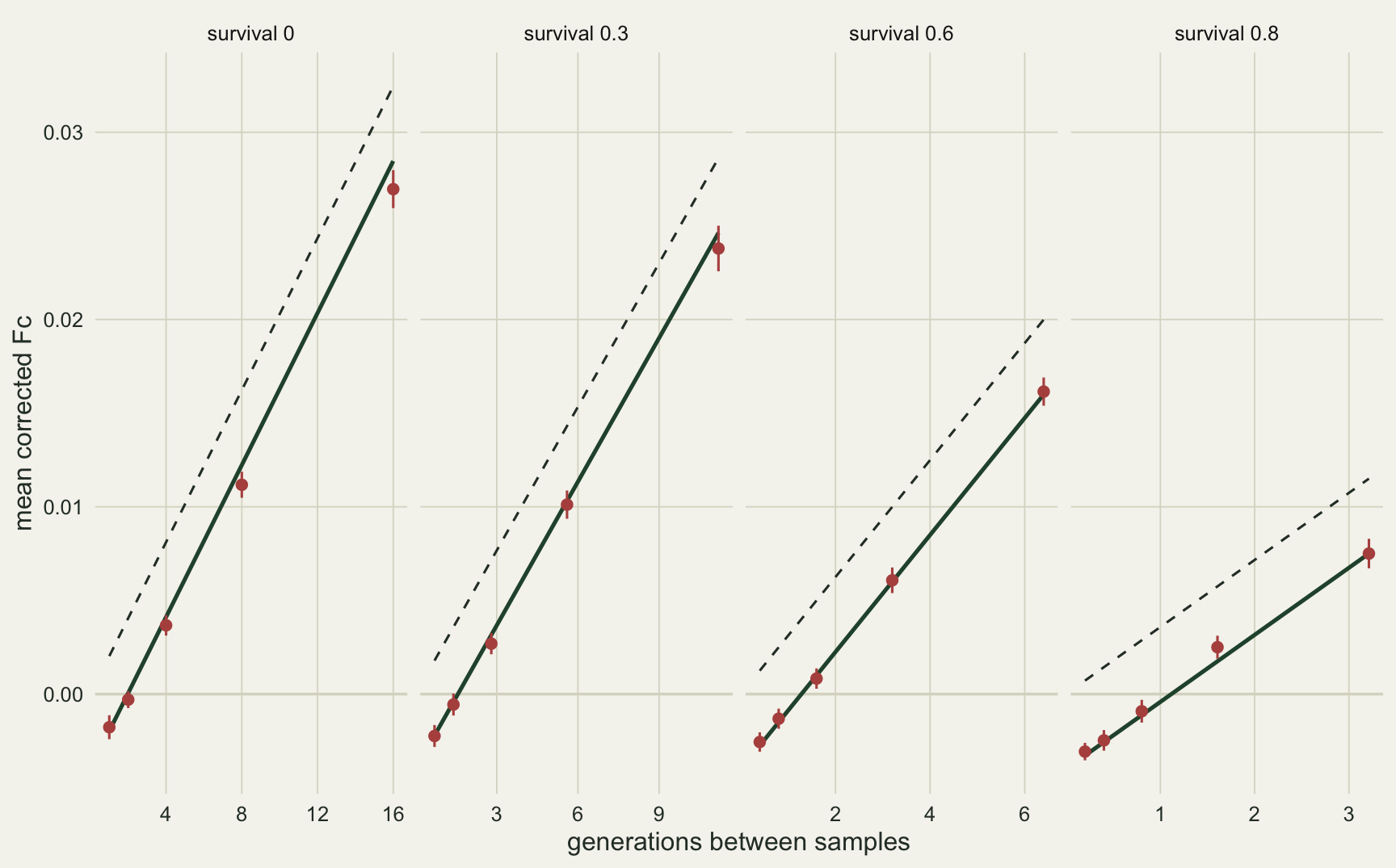
Adding the plan II term back
If the offset is the plan II term, the plan II estimator of Waples 1989, which adds one over the number of adults back to the corrected variance, should remove the bias for both kinds of sample. That needs one extra number from the field, the size of the adult pool, which a count of breeders or a mark recapture estimate supplies.
rep_s <- 0.6
rep_long <- subset(est_all, s == rep_s)
rep_long <- rbind(
  data.frame(gap = rep_long$gap, est = "newborns, standard", r = rep_long$ne_new / rep_long$ne_true),
  data.frame(gap = rep_long$gap, est = "newborns, plan II term", r = rep_long$ne_new_cen / rep_long$ne_true),
  data.frame(gap = rep_long$gap, est = "adults, plan II term", r = rep_long$ne_ad_cen / rep_long$ne_true))
rep_long$est <- factor(rep_long$est, levels = c("newborns, standard", "newborns, plan II term", "adults, plan II term"))
long_ok <- tab_main$gap >= 8
cen_err_long <- max(abs(c(tab_main$med_new_cen[long_ok], tab_main$med_ad_cen[long_ok]) /
                          tab_main$ne_true[long_ok] - 1))
neg_cen_short <- cell(0.8, 1, "neg_ad_cen")
With the plan II term, the median estimate at eight and sixteen years is within 13 per cent of the truth for every life history and both kinds of sample. At a survival of 0.6 and four years the medians are 1.04 of the truth from newborns and 1.04 from adults, where the standard estimator gave 2.0. What the plan II term cannot fix is the lack of drift. One year apart at a survival of 0.8 the median from adults is 0.13 of the truth and 48 per cent of the estimates are still negative: the expected drift in one year is a small fraction of the sampling noise of 50 individuals, and a ratio built on a noisy denominator has a median far from its expectation.
ggplot(rep_long, aes(factor(gap), r, fill = est)) +
  geom_hline(yintercept = 1, linetype = "dashed", colour = te_body) +
  geom_hline(yintercept = 0, colour = te_line) +
  geom_boxplot(outlier.size = 0.6, linewidth = 0.4, colour = te_body) +
  scale_fill_manual(values = c(te_rust, te_gold, te_forest), name = NULL) +
  coord_cartesian(ylim = c(-3, 5)) +
  labs(x = "years between samples", y = "estimate / true Ne") +
  theme_datasheet() + theme(legend.position = "bottom")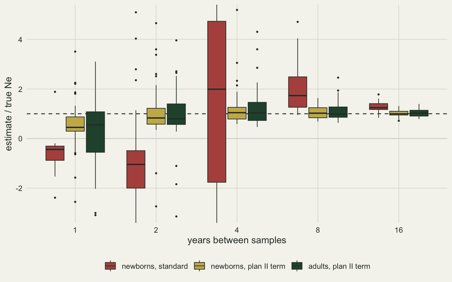
Large cohorts and uneven families change the sign
The plan II result above rests on every sampled newborn recruiting, and a trout is not that. Most newborns die before recruiting, and a few females contribute a large share of each cohort. The two changes are taken one at a time.
With ten newborns per recruit and Poisson families, the same recursion gives an offset of minus one minus survival over the number of newborns for newborn samples, a tenth of the plan II term: only a tenth of the sampled cohort goes on to breed, so the sample sits most of the way towards plan I. Adult samples keep the full plan II term. The chunk runs this at a survival of 0.8, with the same sample of 50, which is now a tenth of its cohort instead of all of it.
juv_u <- 0.1; shape_u <- 0.5; surv_u <- c(0.3, 0.6, 0.8)
set.seed(3109)
bigc_run <- sim_pop(0.8, juv = juv_u)
bigc <- summarise_run(bigc_run)
bigc$n_born <- bigc_run$n_born
big_share <- n_samp / bigc$n_born
tab_b <- do.call(rbind, lapply(split(bigc$est, bigc$est$gap), function(e)
  data.frame(gap = e$gap[1], ratio_new = median(e$ne_new) / bigc$ne_true,
             neg_new = mean(e$f_new < 0),
             z_new = (mean(e$f_new) - (e$gen[1] / (2 * bigc$ne_true) - (1 - 0.8) / bigc$n_born)) /
               (sd(e$f_new) / sqrt(nrow(e))),
             z_ad = (mean(e$f_ad) - (e$gen[1] / (2 * bigc$ne_true) - 1 / n_ad)) /
               (sd(e$f_ad) / sqrt(nrow(e))))))
bcell <- function(g, col) tab_b[[col]][tab_b$gap == g]
drift_b <- bigc$est$gen / (2 * bigc$ne_true)
off_new_b <- mean(bigc$est$f_new - drift_b) * n_ad
off_ad_b  <- mean(bigc$est$f_ad - drift_b) * n_ad
s8 <- tab_main$s == 0.8
off_new_s8 <- mean(tab_main$mean_f_new[s8] - tab_main$drift_f[s8]) * n_ad
tab_b
gap ratio_new neg_new z_new z_ad
1 1 -0.007017638 0.5000000 -1.525180 -0.8935728
2 2 -0.464469561 0.5208333 -3.964915 -0.9563505
4 4 0.992082062 0.1875000 -1.477421 -1.2115347
8 8 1.436462568 0.0000000 -3.271128 -1.7458956
16 16 1.077675139 0.0000000 -1.084574 -1.0795645Averaged over the five intervals, the corrected variance falls short of the drift term by 1.09 times one over the number of adults for adult samples, the full plan II term as predicted, and by 0.27 times for newborn samples, against 0.94 times at the same survival when every newborn recruited. The newborn offset is larger than the predicted tenth, by up to 4.0 Monte Carlo standard errors in single cells; the small sample bias of the standardised variance, which the prediction ignores, is the likely remainder, and the post does not separate it. The medians of the standard estimator on newborns move with the offset but stay noisy: 0.99 of the truth at four years, 1.44 at eight and 1.08 at sixteen, against a negative median at four years when the sample was the whole cohort; one and two years apart they are still negative, -0.01 and -0.46, because there is almost no drift to measure. The sample size does not appear in the predicted offset at all; it only sets the noise around it. What sets the offset is the share of the sampled cohort that recruits, and in the simple life history a cohort that fully recruits is also a small cohort, which is why a sample of fixed size was a large share of it.
The second set of runs adds the other trout feature: each adult’s share of a year’s newborns is drawn from a gamma distribution with shape 0.5, redrawn every year, so family sizes are strongly overdispersed.
The same recursion now gives a different sign. The newborn deviation e has a larger variance, one over twice the number of newborns plus one over twice the shape times the number of adults, while the finite cohort term shrinks with the size of the cohort. The expected corrected variance for newborn samples becomes the drift term plus 2 s var(e) minus one over the number of newborns, which is positive for these settings, so the standard estimator should now underestimate. Adult samples are unaffected: their expectation is still the drift term minus one over the number of adults, because each adult carries the same weight in the next year’s breeding whatever its age.
set.seed(3108)
sums_u <- lapply(surv_u, function(s) summarise_run(sim_pop(s, juv = juv_u, shape = shape_u)))
tab_u <- do.call(rbind, lapply(sums_u, function(x) {
  do.call(rbind, lapply(split(x$est, x$est$gap), function(e) {
    n_born <- round(round(n_ad * (1 - e$s[1])) / juv_u)
    v_e <- 1 / (2 * n_born) + 1 / (2 * shape_u * n_ad)
    data.frame(s = e$s[1], gap = e$gap[1], ne_true = x$ne_true, gen_time = x$gen_time,
               med_new = median(e$ne_new), med_new_cen = median(e$ne_new_cen),
               med_ad_cen = median(e$ne_ad_cen), neg_ad_cen = mean(e$f_ad + 1 / n_ad < 0),
               mean_f_new = mean(e$f_new), se_f_new = sd(e$f_new) / sqrt(nrow(e)),
               mean_f_ad = mean(e$f_ad), se_f_ad = sd(e$f_ad) / sqrt(nrow(e)),
               pred_new = e$gen[1] / (2 * x$ne_true) + 2 * e$s[1] * v_e - 1 / n_born,
               pred_ad = e$gen[1] / (2 * x$ne_true) - 1 / n_ad)
  }))
}))
ucell <- function(s, g, col) tab_u[[col]][tab_u$s == s & tab_u$gap == g]
uratio <- function(s, g, col) ucell(s, g, col) / ucell(s, g, "ne_true")
z_u_new <- max(abs((tab_u$mean_f_new - tab_u$pred_new) / tab_u$se_f_new))
z_u_ad  <- max(abs((tab_u$mean_f_ad - tab_u$pred_ad) / tab_u$se_f_ad))
ne_u <- vapply(sums_u, `[[`, 0, "ne_true")
inc_u <- surv_u * (1 - surv_u) / (2 * n_ad) +
  (1 - surv_u)^2 * (1 / (2 * round(n_ad * (1 - surv_u))) + 1 / (2 * shape_u * n_ad))
ne_u_an <- (1 - surv_u) / (2 * inc_u)
ne_u_gap <- max(abs(ne_u / ne_u_an - 1))
The true effective sizes drop to 93, 105 and 115 at survivals of 0.3, 0.6 and 0.8, within 1 per cent of the value from the yearly variance recursion. The predicted mean variances hold within 3.8 standard errors for newborn samples and 2.2 for adult samples; the newborn prediction uses a large pool approximation for the gamma weights, so a slightly looser fit there is not a surprise.
The standard estimator on newborns now errs downward. At a survival of 0.3 it recovers by eight years (1.02 of the truth), but at a survival of 0.6 the median one year apart is 0.31 of the truth, four years apart 0.74 and sixteen years apart 0.91; at a survival of 0.8 sixteen years apart it is still 0.75. Adding the plan II term makes the newborn estimates worse, 0.81 at 0.6 and sixteen years, because the term it removes is no longer the one that is there. Adult samples with the plan II term give 1.04 and 1.05 of the truth at eight and sixteen years at a survival of 0.6, the same behaviour as in the simple life history, including the same shortfall at short intervals (0.34 one year apart at a survival of 0.8).
This is the direction Waples and Yokota 2007 describe: whether newborn or adult samples bias the temporal estimate up or down depends on the life history, and the rate of change conforms to the discrete generation model only when individuals are weighted by reproductive value. Here survival and fecundity do not depend on age, every adult has the same reproductive value, and a random sample of adults is already correctly weighted, which is why the adult sample with the plan II term works in both life histories. Jorde and Ryman 1995 built the other route, a correction factor for change between cohorts computed from age specific survival and birth rates. That factor is not reproduced in this post; the newborn correction used above is derived for these two toy life histories only, and what it shares with theirs is the direction of the argument: a newborn sample cannot be corrected without the life table and the variance of family size.
u_long <- rbind(
  data.frame(s = tab_u$s, gap = tab_u$gap, est = "newborns, standard", r = tab_u$med_new / tab_u$ne_true),
  data.frame(s = tab_u$s, gap = tab_u$gap, est = "newborns, plan II term", r = tab_u$med_new_cen / tab_u$ne_true),
  data.frame(s = tab_u$s, gap = tab_u$gap, est = "adults, plan II term", r = tab_u$med_ad_cen / tab_u$ne_true))
u_long$est <- factor(u_long$est, levels = c("newborns, standard", "newborns, plan II term", "adults, plan II term"))
u_long$surv_lab <- paste("survival", u_long$s)
ggplot(u_long, aes(gap, r, colour = est)) +
  geom_hline(yintercept = 1, linetype = "dashed", colour = te_body) +
  geom_line(linewidth = 0.8) + geom_point(size = 2) +
  scale_x_log10(breaks = gaps) +
  scale_colour_manual(values = c(te_rust, te_gold, te_forest), name = NULL) +
  facet_wrap(~ surv_lab, nrow = 1) +
  labs(x = "years between samples", y = "median estimate / true Ne") +
  theme_datasheet() + theme(legend.position = "bottom")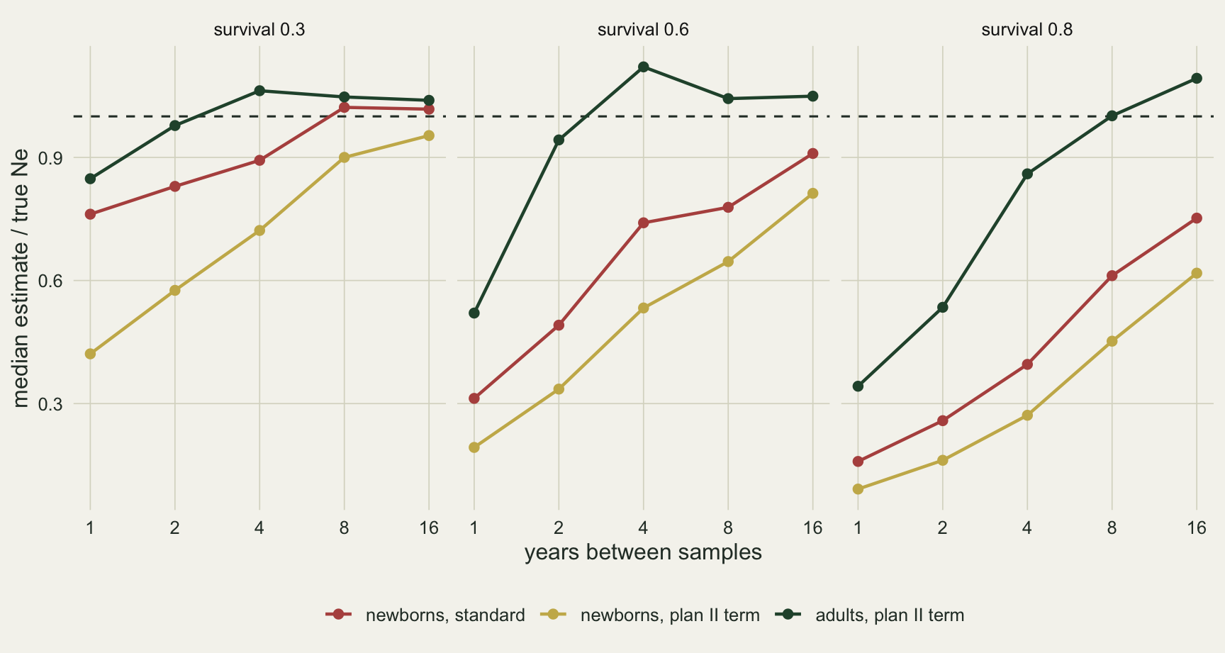
What to report
Say which individuals were sampled, newborns of one cohort, adults, or a mix of ages, and how the cohort or pool was defined. The same allele frequency change means a different effective size under each: with ten newborns per recruit and uneven families, at a survival of 0.6 and eight years apart, newborn samples gave 0.78 of the truth and adult samples with the plan II term 1.04.
Give the interval in years and the generation time used to turn it into generations, with its source. The estimate scales directly with that generation time, and a generation time taken from a life table for a different population is a second estimate hidden inside the first.
Report the share of negative or infinite estimates in any resampling or jackknife, and the median, rather than dropping the negative ones and averaging the rest. A negative estimate one or two years apart is not an estimate of a very large population; in these runs it was the expected outcome for a population of known, modest size.
If the adult census size is known, show the plan I estimate and the plan II estimate of Waples 1989 side by side, and say whether the samples were taken with replacement or from a finite pool. For a sample of adults in a population whose survival and fecundity do not change much with age, the plan II estimate is the one to trust. For newborns, give the size of the sampled cohort, the share of it the sample was, and the share expected to recruit; a sample from a cohort that wholly recruits is a plan II sample whatever its size, and a sample from a large cohort of which few recruit is closer to plan I. Where family sizes are uneven, say that the correction also depends on juvenile mortality and family size variance, and give the life table values used; a correction without them is a guess about their direction.
Prefer intervals of several generations when the archive allows it. Every repair above gets better with the drift signal, and none of them rescues one or two years.
Honest limits
Survival and fecundity do not depend on age in either life history. That is the case in which adults all carry the same reproductive value, and it is the reason a random adult sample works. A species that matures late, or whose fecundity rises with size, gives older adults more weight in the next cohorts, and a random adult sample is then no longer correctly weighted; the adult result here should not be carried to such species without rerunning the code with an age schedule.
The population is constant in size, closed, and breeds at random with selfing allowed. Changing size makes the truth a harmonic mean over the interval and moves the plan II term with it; migration adds allele frequency change that the estimator reads as drift.
The newborn correction for large cohorts and uneven families uses an approximation for the gamma weights, and it is a correction derived here for this model, not the Jorde and Ryman factor. Its fit to the simulated mean was looser than for the simple life history, and it needs quantities (juvenile survival, the shape of the family size distribution) that are rarely known for a wild population.
The replicates share their first sample across the five intervals, so the five cells of one life history are not independent, and with 48 replicates per cell a share of negative estimates carries a Monte Carlo standard error of up to 7.2 percentage points. The loci are unlinked and neutral and the samples carry no genotyping error. The effective size is the inbreeding effective size from the decay of heterozygosity; with a constant population the variance effective size is expected to agree, but that was not measured separately.
References
Nei M, Tajima F 1981 Genetics 98(3):625-640 (10.1093/genetics/98.3.625)
Waples RS 1989 Genetics 121(2):379-391 (10.1093/genetics/121.2.379)
Hill WG 1979 Genetics 92(1):317-322 (10.1093/genetics/92.1.317)
Jorde PE, Ryman N 1995 Genetics 139(2):1077-1090 (10.1093/genetics/139.2.1077)
Waples RS, Yokota M 2007 Genetics 175(1):219-233 (10.1534/genetics.106.065300)