library(ggplot2)

te_paper  <- "#f5f4ee"
te_ink    <- "#16241d"
te_body   <- "#2c3a31"
te_forest <- "#275139"
te_rust   <- "#b5534e"
te_gold   <- "#c9b458"
te_line   <- "#dad9ca"

theme_datasheet <- function() {
  theme_minimal(base_size = 12) +
    theme(plot.background  = element_rect(fill = te_paper, colour = NA),
          panel.background = element_rect(fill = te_paper, colour = NA),
          panel.grid.major = element_line(colour = te_line, linewidth = 0.3),
          panel.grid.minor = element_blank(),
          text             = element_text(colour = te_body),
          plot.title       = element_text(colour = te_ink, face = "bold"),
          plot.subtitle    = element_text(colour = te_body),
          axis.text        = element_text(colour = te_body))
}Purging siblings before estimating Ne
R
population genetics
effective population size
simulation
ecology tutorial
ggplot2
Removing putative siblings from a random sample inflates a linkage disequilibrium estimate of effective size several fold. A simulation of the purge in R.
A stream has been sampled for juvenile brown trout, a hundred fish are genotyped at a SNP panel, and the genotypes go into a sibship reconstruction program before anything else happens. The program returns a list of full sib and half sib pairs, and the workflow note attached to the project says what every workflow note says: remove siblings before running the effective size estimator, because the estimator assumes a random sample of unrelated individuals. One fish per reconstructed family goes forward, half of them are dropped, and the estimate comes back three times larger than the one from the whole sample. The larger number is the one that goes in the report, because it came from the cleaner data set.
It is the wrong number, and the direction of the error is the opposite of what the workflow note was guarding against. The estimator does assume a random sample of unrelated individuals, but in a randomly sampled cohort that assumption is not violated by the presence of siblings. A random sample of a hundred juveniles from a population whose effective size is a hundred contains siblings in a quantity that is fixed by the effective size itself, and the linkage disequilibrium method reads exactly that quantity. Conditioning the sample on the absence of shared parents removes the signal the method exists to measure.
This post is the other half of a result the site already has in one direction. Checking an effective size estimate builds samples on purpose as a few families of many offspring, shows the estimate collapsing from 327 to 15 as the families get larger, and ends with the usual advice: relatedness screening before estimation, or one individual per family, or a method that models the family structure. That advice is for a sample built from families. Applied to a randomly sampled cohort it manufactures the opposite error, and the measurements below say by how much. The estimator itself is the one from estimating Ne from genetic data, permutation floor and all, and the quantity being estimated is the one from effective population size: the Crow and Kimura expression in the family size variance.
The result is not new. Waples and Anderson set it out in 2017 as a cautionary view on purging putative siblings, and what follows is a demonstration of it with the site’s own generator. What the simulation adds is a same size random control beside every purged estimate, so that conditioning is separated from small sample noise, and a purge rule sweep that answers the two questions a practitioner asks next.
The siblings in a random sample are the estimate
The generator is the hermaphrodite Wright-Fisher population used throughout the effective size posts here: a fixed number of adults, selfing allowed, and every offspring drawing two gametes from the adult pool with probabilities proportional to a per adult fecundity weight. The weights are gamma draws with mean one, and the shape parameter is the single knob that sets how uneven reproduction is. An infinite shape gives equal weights and Poisson family sizes, so the effective size sits near the census. A shape of one, and then of a quarter, push it down.
The true effective size of a realised run is not assumed, it is counted. Each generation the number of gametes contributed by each adult is recorded, its variance across adults is the family size variance, and the Crow and Kimura expression turns that into a per generation effective size. The linkage disequilibrium signal comes from the last handful of generations, so the truth used below is the harmonic mean of the per generation values over the last six.
one_gen <- function(hap, n_adult, n_locus, shape) {
  wt <- if (is.finite(shape)) rgamma(n_adult, shape, shape) else rep(1, n_adult)
  pa <- sample(n_adult, n_adult, replace = TRUE, prob = wt)
  pb <- sample(n_adult, n_adult, replace = TRUE, prob = wt)
  pick <- function(par) {
    rows <- 2 * par - 1 + matrix(sample(0:1, n_adult * n_locus, TRUE),
                                 n_adult, n_locus)
    matrix(hap[cbind(as.vector(rows), rep(seq_len(n_locus), each = n_adult))],
           n_adult, n_locus)
  }
  kid <- matrix(0L, 2 * n_adult, n_locus)
  kid[seq(1, 2 * n_adult, 2), ] <- pick(pa)
  kid[seq(2, 2 * n_adult, 2), ] <- pick(pb)
  list(hap = kid, pa = pa, pb = pb, vk = var(tabulate(c(pa, pb), n_adult)))
}

sim_pop <- function(n_adult, shape, gens = 25, n_locus = 120) {
  p0  <- runif(n_locus, 0.2, 0.8)
  hap <- matrix(rbinom(2 * n_adult * n_locus, 1, rep(p0, each = 2 * n_adult)),
                2 * n_adult)
  vk_gen <- numeric(gens)
  for (g in seq_len(gens)) {
    hap_par <- hap
    step    <- one_gen(hap, n_adult, n_locus, shape)
    hap     <- step$hap
    vk_gen[g] <- step$vk
  }
  ne_gen <- (4 * n_adult - 2) / (vk_gen + 2)
  list(hap = hap, hap_par = hap_par, pa = step$pa, pb = step$pb,
       ne_true = 1 / mean(1 / ne_gen[(gens - 5):gens]), ne_last = ne_gen[gens])
}
The estimator is the one from the earlier post, built on the unlinked loci relation of Hill 1981. The mean squared correlation between unlinked loci is measured on the sample, the sampling floor is measured by permuting alleles among individuals within each locus, and the effective size is one over three times the difference. Measuring the floor by permutation stands in for the analytic bias correction of Waples 2006 that the applied estimates surveyed by Waples and Do 2010 use. Loci with a minor allele frequency below five per cent in the sample are dropped, which is the usual filter and matters here because the purged subsets are small.
A sample whose observed correlation falls below its own permutation floor returns an infinite value, which is not a large estimate but no estimate. Every median below is taken over the replicates that returned a finite value, and the number that did not is reported beside it.
mean_r2 <- function(hap, maf_min = 0.05) {
  frq  <- colMeans(hap)
  keep <- pmin(frq, 1 - frq) >= maf_min
  cr   <- suppressWarnings(cor(hap[, keep, drop = FALSE]))
  r2   <- cr[upper.tri(cr)]^2
  mean(r2[is.finite(r2)])
}

ld_ne <- function(hap_s, n_perm = 4) {
  obs <- mean_r2(hap_s)
  flr <- mean(replicate(n_perm, mean_r2(apply(hap_s, 2, sample))))
  gap <- obs - flr
  if (!is.finite(gap) || gap <= 0) Inf else 1 / (3 * gap)
}

take <- function(hap, ids) hap[as.vector(rbind(2 * ids - 1, 2 * ids)), ,
                               drop = FALSE]

med_fin <- function(v) median(v[is.finite(v)])
n_fail  <- function(v) sum(!is.finite(v))
Before any purging, count what is there. For two offspring drawn at random, look at the four ways of pairing one of the first one’s two parents with one of the second one’s two parents, and count how many of those four pairings land on the same adult. Full siblings score two, half siblings score one, unrelated pairs score zero, and two offspring of the same selfing adult score four. The expected score is four times the probability that two random gametes came from the same adult, and that probability is one over the effective size, because it is the same probability the Crow and Kimura expression is built from. So the mean shared parent count over the pairs of a random sample estimates four over Ne, and four over that count is an estimate of Ne in its own right. It is the quantity the sibship frequency estimator of Wang uses, and it is exactly what the purge throws away.
shared_count <- function(ids, pa, pb) {
  a <- pa[ids]; b <- pb[ids]
  m <- outer(a, a, "==") + outer(a, b, "==") +
       outer(b, a, "==") + outer(b, b, "==")
  m[upper.tri(m)]
}
Two purge rules are needed. The first keeps one member of each reconstructed full sib family and drops the rest, which is what a sibship program’s family list supports directly. The second is the rule the workflow notes describe, one individual per family with half siblings counted as family: walk the sample in its (random) order, keep an individual only if neither of its parents has already been claimed by a kept individual, and drop it otherwise. The second rule is the greedy first come purge, and it is the one that does the damage.
purge_full <- function(ids, pa, pb) {
  key <- paste(pmin(pa[ids], pb[ids]), pmax(pa[ids], pb[ids]), sep = "-")
  ids[!duplicated(key)]
}

purge_half <- function(ids, pa, pb) {
  claimed <- logical(max(c(pa, pb)))
  keep    <- logical(length(ids))
  for (i in seq_along(ids)) {
    par_a <- pa[ids[i]]; par_b <- pb[ids[i]]
    if (!claimed[par_a] && !claimed[par_b]) {
      keep[i] <- TRUE
      claimed[par_a] <- TRUE
      claimed[par_b] <- TRUE
    }
  }
  ids[keep]
}
The grid below crosses three fecundity shapes with two sampling fractions and two census sizes, twelve replicate populations per cell. Everything about the design was fixed before the first run: twenty five generations, a hundred and twenty unlinked loci, four permutations for the floor, and twelve replicates. Each replicate produces four estimates from the same population and the same initial sample: the whole sample, the full sib purge, the half and full sib purge, and a random subsample of the size the half sib purge left. That last one is the control, and without it none of the rest can be read.
run_cell <- function(n_adult, n_sample, shape, n_rep = 12) {
  out <- NULL
  for (r in seq_len(n_rep)) {
    pop <- sim_pop(n_adult, shape)
    ids <- sample(n_adult, n_sample)
    k_f <- purge_full(ids, pop$pa, pop$pb)
    k_h <- purge_half(ids, pop$pa, pop$pb)
    ctl <- sample(ids, length(k_h))
    mlt <- shared_count(ids, pop$pa, pop$pb)
    out <- rbind(out, data.frame(
      rep_id = r, ne_true = pop$ne_true, ne_last = pop$ne_last,
      mean_shared = mean(mlt), sib_share = mean(mlt > 0),
      ne_sib = 4 / mean(mlt), kept_full = length(k_f), kept_half = length(k_h),
      ne_all = ld_ne(take(pop$hap, ids)), ne_pf = ld_ne(take(pop$hap, k_f)),
      ne_ph = ld_ne(take(pop$hap, k_h)), ne_ct = ld_ne(take(pop$hap, ctl))))
  }
  out
}

set.seed(20492)
cells <- expand.grid(shape = c(Inf, 1, 0.25), frac = c(0.2, 0.5),
                     n_adult = c(200, 500))
all_rep <- do.call(rbind, lapply(seq_len(nrow(cells)), function(i) {
  cf <- cells[i, ]
  res <- run_cell(cf$n_adult, round(cf$n_adult * cf$frac), cf$shape)
  cbind(res, n_adult = cf$n_adult, frac = cf$frac, shape = cf$shape,
        n_samp = round(cf$n_adult * cf$frac))
}))

n_rep_tot  <- nrow(all_rep)
sib_ratio  <- median(all_rep$ne_sib / all_rep$ne_true)
sib_last   <- median(all_rep$ne_sib / all_rep$ne_last)
sib_lo     <- quantile(all_rep$ne_sib / all_rep$ne_true, 0.25)
sib_hi     <- quantile(all_rep$ne_sib / all_rep$ne_true, 0.75)
share_pct  <- 100 * median(all_rep$sib_share)
by_shape   <- tapply(all_rep$sib_share, all_rep$shape, median)
share_flat <- 100 * by_shape[["Inf"]]
share_skew <- 100 * by_shape[["0.25"]]
ne_span    <- max(all_rep$ne_true) / min(all_rep$ne_true)
kept_pct   <- 100 * median(all_rep$kept_half / all_rep$n_samp)
rm_full_md <- median(all_rep$n_samp - all_rep$kept_full)
rm_full_hi <- max(all_rep$n_samp - all_rep$kept_full)
Across all 144 replicates the median share of sample pairs that are full or half siblings is 2.6 per cent, from 1.2 per cent with equal fecundity weights to 5.0 per cent at the strongest skew. Those pairs are not contamination. Four divided by the mean shared parent count recovers the realised effective size with a median ratio of 1.028 and a quartile range of 0.935 to 1.107, over populations whose true effective size spans a factor of 15. That ratio is against the six generation harmonic mean; against the single parental generation value, which is what the shared parent count of a sampled cohort measures directly, the median ratio is 1.006. The pedigree information in the sample is a calibrated measurement of the thing the study is trying to measure.
The two rules remove very different amounts. The full sib purge drops a median of 0 individuals and never more than 13, because two offspring of the same parent pair are rare when parents pair at random. The half sib purge keeps 46.5 per cent of the sample, so it throws away about half of it. The difference between those two rules is the whole story of the next section.
sib_df <- data.frame(ne_true = all_rep$ne_true, ne_sib = all_rep$ne_sib,
                     shape = factor(all_rep$shape,
                                    levels = c(Inf, 1, 0.25),
                                    labels = c("equal weights", "gamma shape 1",
                                               "gamma shape 0.25")))

ggplot(sib_df, aes(ne_true, ne_sib, colour = shape)) +
  geom_abline(slope = 1, intercept = 0, linetype = "dashed",
              colour = te_body, linewidth = 0.6) +
  geom_point(size = 1.9, alpha = 0.85) +
  scale_x_log10() +
  scale_y_log10() +
  scale_colour_manual(values = c(te_gold, te_forest, te_rust), name = NULL) +
  labs(x = "realised effective size", y = "four over the mean shared parent count",
       title = "The siblings are a measurement, not contamination",
       subtitle = "one point per replicate; dashed line: equality") +
  theme_datasheet() +
  theme(legend.position = "bottom")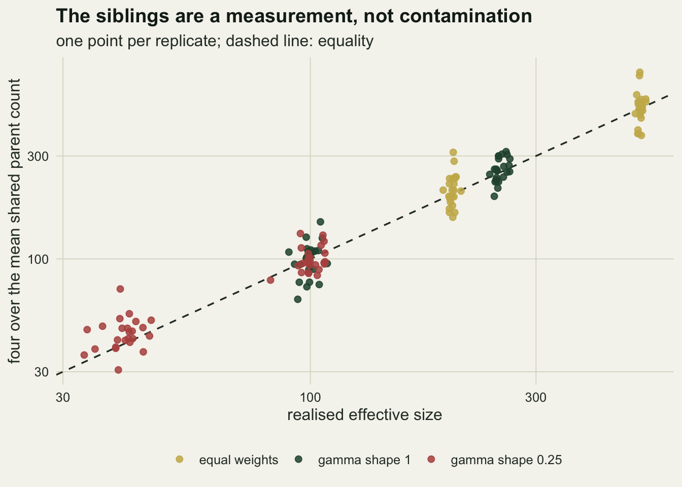
What the purge does
Four numbers per replicate, all from the same population and the same initial sample of individuals, divided by that replicate’s own realised effective size. The whole sample is the baseline, the two purge rules are the treatments, and the random subsample of the purged size is the control that separates conditioning from the loss of individuals.
ratio_tab <- data.frame(
  shape = all_rep$shape, n_adult = all_rep$n_adult, frac = all_rep$frac,
  all    = all_rep$ne_all / all_rep$ne_true,
  purgeF = all_rep$ne_pf  / all_rep$ne_true,
  purgeH = all_rep$ne_ph  / all_rep$ne_true,
  ctrl   = all_rep$ne_ct  / all_rep$ne_true)

med_by <- function(v) {
  tapply(v, list(ratio_tab$n_adult, ratio_tab$frac, ratio_tab$shape), med_fin)
}
med_all  <- med_by(ratio_tab$all)
med_pf   <- med_by(ratio_tab$purgeF)
med_ph   <- med_by(ratio_tab$purgeH)
med_ct   <- med_by(ratio_tab$ctrl)

r_all_lo <- min(med_all); r_all_hi <- max(med_all)
r_pf_lo  <- min(med_pf);  r_pf_hi  <- max(med_pf)
r_ph_lo  <- min(med_ph);  r_ph_hi  <- max(med_ph)
r_ct_lo  <- min(med_ct);  r_ct_hi  <- max(med_ct)

pair_ok  <- is.finite(all_rep$ne_ph) & is.finite(all_rep$ne_ct)
n_paired <- sum(pair_ok)
n_beat   <- sum(all_rep$ne_ph[pair_ok] > all_rep$ne_ct[pair_ok])
fold     <- (all_rep$ne_ph / all_rep$ne_ct)[pair_ok]
fold_md  <- median(fold)
fold_lo  <- quantile(fold, 0.25)
fold_hi  <- quantile(fold, 0.75)
n_inf_ph <- n_fail(all_rep$ne_ph)
n_inf    <- n_inf_ph + n_fail(all_rep$ne_ct) + n_fail(all_rep$ne_all)
fail_hi  <- 1 - 0.05^(1 / n_paired)
ctl_off  <- 100 * max(abs(c(r_ct_lo, r_ct_hi) - 1))
pc_lo    <- min(med_ph / med_ct); pc_hi <- max(med_ph / med_ct)
win_gap  <- median(all_rep$ne_true / all_rep$ne_last)
ph_last  <- med_fin(all_rep$ne_ph / all_rep$ne_last)
ph_six   <- med_fin(all_rep$ne_ph / all_rep$ne_true)
row_pick <- ratio_tab$n_adult == 200 & ratio_tab$frac == 0.5 &
            ratio_tab$shape == 1
ex_all <- med_fin(ratio_tab$all[row_pick]); ex_ph <- med_fin(ratio_tab$purgeH[row_pick])
ex_ct  <- med_fin(ratio_tab$ctrl[row_pick])
The whole sample estimate is close to the realised effective size everywhere: the per cell median ratio runs from 0.89 to 1.16. The full sib purge is the same estimate with a handful of individuals missing, and its per cell median ratio runs from 0.91 to 1.19. The half and full sib purge, the rule the workflow notes actually describe, gives per cell median ratios from 3.69 to 4.94.
The control settles what that means. A random subsample of the same size, drawn from the same forty, hundred or two hundred and fifty individuals, gives per cell median ratios from 0.94 to 1.40. The individuals lost to the purge are not the problem. Within a replicate, the purged estimate exceeded its own same size control in every replicate in which both returned a finite estimate, 139 of the 144; in the other 5 the purged sample fell below the permutation floor and returned infinity, which is the same failure in a stronger form. With no exceptions in 139 paired draws the upper 95 per cent bound on the rate of exceptions is 0.021, so the sign of the effect is not in doubt and the remaining question is its size: the median ratio of purged estimate to its own control is 3.5, with a quartile range of 2.5 to 5.4. The cell nearest to a real study, two hundred adults, half of them sampled and a fecundity shape of one, reads 1.08 for the whole sample, 1.11 for the random control and 3.80 for the purged set.
lvl <- c("equal weights", "gamma shape 1", "gamma shape 0.25")
long_med <- do.call(rbind, lapply(
  list(c("all", "whole sample"), c("purgeF", "full sib purge"),
       c("purgeH", "half and full sib purge"), c("ctrl", "random control")),
  function(nm) {
    m <- tapply(ratio_tab[[nm[1]]],
                list(ratio_tab$n_adult, ratio_tab$frac, ratio_tab$shape), med_fin)
    dn <- dimnames(m)
    gg <- expand.grid(n_adult = dn[[1]], frac = dn[[2]], shape = dn[[3]],
                      stringsAsFactors = FALSE)
    data.frame(gg, ratio = as.vector(m), rule = nm[2])
  }))
long_med$shape <- factor(long_med$shape, levels = c("Inf", "1", "0.25"),
                         labels = lvl)
long_med$rule  <- factor(long_med$rule,
                         levels = c("half and full sib purge", "whole sample",
                                    "full sib purge", "random control"))
long_med$panel <- sprintf("%s adults, %s sampled", long_med$n_adult,
                          ifelse(long_med$frac == "0.2", "a fifth", "a half"))

ggplot(long_med, aes(shape, ratio, colour = rule, group = rule)) +
  geom_hline(yintercept = 1, linetype = "dashed", colour = te_body,
             linewidth = 0.6) +
  geom_line(aes(linetype = rule), linewidth = 0.8) +
  geom_point(aes(shape = rule), size = 2.6) +
  facet_wrap(~ panel) +
  scale_y_log10(breaks = c(0.5, 1, 2, 5, 10)) +
  scale_colour_manual(values = c(te_rust, te_gold, te_forest, te_body),
                      name = NULL) +
  scale_linetype_manual(values = c("solid", "solid", "solid", "22"),
                        name = NULL) +
  scale_shape_manual(values = c(16, 16, 16, 1), name = NULL) +
  labs(x = "fecundity weights", y = "median estimate over realised Ne",
       title = "Only the purged sample leaves the truth",
       subtitle = "twelve replicate populations per cell; dashed line: the realised effective size") +
  theme_datasheet() +
  theme(legend.position = "bottom", axis.text.x = element_text(size = 8))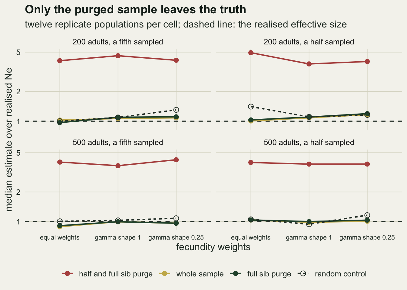
The purge rule and the identification error do not rescue it
Two questions come straight back. The greedy walk above keeps whoever comes first, which is an arbitrary rule; does a different one behave differently? And a real sibship program does not hand over the true pedigree, it hands over a reconstruction with errors in it; do false sibling pairs dilute the effect?
Both are answered on one set of populations, two hundred adults and a sample of a hundred, at the two fecundity shapes where the estimator has something to work with. The purge is rewritten to operate on a pair list rather than on parent identities, which is the form a program’s output actually takes, so that pairs can be added to it or taken out of it. Three rules are compared: the greedy walk in sample order, the greedy walk in a second random order, and one randomly chosen individual per connected group of the sibling graph, which is the strictest reading of one individual per family. Two error levels add false pairs at five and ten per cent of the true pair count, and one level deletes a fifth of the true pairs. Every variant gets its own same size random control.
sib_adj <- function(ids, pa, pb) {
  a <- pa[ids]; b <- pb[ids]
  adj <- outer(a, a, "==") | outer(a, b, "==") |
         outer(b, a, "==") | outer(b, b, "==")
  diag(adj) <- FALSE
  adj
}

greedy_adj <- function(adj, ord = seq_len(nrow(adj))) {
  keep <- integer(0)
  for (i in ord) if (!any(adj[i, keep])) keep <- c(keep, i)
  sort(keep)
}

one_per_group <- function(adj) {
  n <- nrow(adj); lab <- integer(n); cur <- 0L
  for (i in seq_len(n)) if (lab[i] == 0L) {
    cur <- cur + 1L; stack <- i
    while (length(stack)) {
      v <- stack[1]; stack <- stack[-1]
      if (lab[v] == 0L) { lab[v] <- cur; stack <- c(stack, which(adj[v, ] & lab == 0L)) }
    }
  }
  as.integer(vapply(split(seq_len(n), lab),
                    function(v) if (length(v) == 1) v else sample(v, 1), 1L))
}

perturb <- function(adj, add_rate = 0, drop_rate = 0) {
  ut <- which(upper.tri(adj))
  is_pair <- adj[ut]
  n_true  <- sum(is_pair)
  if (drop_rate > 0 && n_true > 0) {
    gone <- sample(ut[is_pair], round(drop_rate * n_true))
    adj[gone] <- FALSE
  }
  if (add_rate > 0 && n_true > 0) {
    new <- sample(ut[!is_pair], round(add_rate * n_true))
    adj[new] <- TRUE
  }
  adj | t(adj)
}

set.seed(51190)
rule_rows <- NULL
for (sh in c(1, 0.25)) {
  for (r in 1:12) {
    pop <- sim_pop(200, sh)
    ids <- sample(200, 100)
    adj <- sib_adj(ids, pop$pa, pop$pb)
    sets <- list(
      "greedy, sample order"    = greedy_adj(adj),
      "greedy, second order"    = greedy_adj(adj, sample(nrow(adj))),
      "one per sibling group"   = one_per_group(adj),
      "greedy, 5% false pairs"  = greedy_adj(perturb(adj, add_rate = 0.05)),
      "greedy, 10% false pairs" = greedy_adj(perturb(adj, add_rate = 0.10)),
      "greedy, a fifth missed"  = greedy_adj(perturb(adj, drop_rate = 0.20)))
    for (nm in names(sets)) {
      kept <- ids[sets[[nm]]]
      rule_rows <- rbind(rule_rows, data.frame(
        shape = sh, rep_id = r, rule = nm, n_kept = length(kept),
        purged = ld_ne(take(pop$hap, kept)) / pop$ne_true,
        control = ld_ne(take(pop$hap, sample(ids, length(kept)))) / pop$ne_true))
    }
  }
}

rule_med <- aggregate(cbind(purged, control, n_kept) ~ rule + shape,
                      data = rule_rows, FUN = med_fin)
g1 <- rule_med$rule == "greedy, sample order"
g2 <- rule_med$rule == "greedy, second order"
gg_gap  <- max(abs(rule_med$purged[g1] - rule_med$purged[g2]))
grp_n   <- rule_med$n_kept[rule_med$rule == "one per sibling group"]
err_set <- c("greedy, 5% false pairs", "greedy, 10% false pairs")
err_lo  <- min(rule_med$purged[rule_med$rule %in% err_set])
err_hi  <- max(rule_med$purged[rule_med$rule %in% err_set])
base_lo <- min(rule_med$purged[g1]); base_hi <- max(rule_med$purged[g1])
miss_lo <- min(rule_med$purged[rule_med$rule == "greedy, a fifth missed"])
miss_hi <- max(rule_med$purged[rule_med$rule == "greedy, a fifth missed"])
grp_row <- rule_rows$rule == "one per sibling group"
keep_rule <- rule_med$rule != "one per sibling group"
ctrl_hi <- max(rule_med$control[keep_rule])
grp_inf <- n_fail(rule_rows$purged[grp_row]) + n_fail(rule_rows$control[grp_row])
grp_n_tot <- 2 * sum(grp_row)
rule_inf  <- n_fail(rule_rows$purged) + n_fail(rule_rows$control)
rule_est  <- 2 * nrow(rule_rows)
min_gap <- min(rule_med$purged[keep_rule] / rule_med$control[keep_rule])
The order of the greedy walk is not what drives the result. The sample order rule gives median ratios of 3.9 and 4.7 in the two fecundity cells, and a second random order differs from it by at most 0.81. Both sit several times above their own controls, twelve replicates cannot resolve a difference of that size, and nothing in the mechanism suggests one.
The strict rule is a different matter, and it is not a rival estimate. One randomly chosen individual per connected sibling group keeps a median of 3 to 9 individuals out of a hundred, because the shared parent graph of a sample that size is mostly one large connected component. At that size the estimator has nothing to work with: 12 of the 48 estimates it produces, purged sets and controls together, fall below the permutation floor and come back infinite. The strict reading of one individual per family does not give a worse estimate, it gives no estimate.
Identification error does not dilute the effect either. With false pairs at five and ten per cent of the true pair count the median ratio is between 3.7 and 5.1, against 3.9 to 4.7 with a perfect pair list, and missing a fifth of the true pairs gives 4.1 to 4.7. Every one of the five greedy variants sits more than three times above its own same size control, the smallest of those ratios being 3.19, and the largest control median across the ten cells is 1.31 times the truth. A sibship program that makes mistakes still purges the drift signal, because the signal is carried by the pairs it gets right.
plot_med  <- rule_med[keep_rule, ]
rule_long <- rbind(
  data.frame(rule = plot_med$rule, shape = plot_med$shape,
             ratio = plot_med$purged, kind = "purged set"),
  data.frame(rule = plot_med$rule, shape = plot_med$shape,
             ratio = plot_med$control, kind = "random control, same size"))
ord <- c("greedy, sample order", "greedy, second order",
         "greedy, 5% false pairs", "greedy, 10% false pairs",
         "greedy, a fifth missed")
rule_long$rule  <- factor(rule_long$rule, levels = rev(ord))
rule_long$panel <- factor(rule_long$shape, levels = c(1, 0.25),
                          labels = c("gamma shape 1", "gamma shape 0.25"))

ggplot(rule_long, aes(ratio, rule, colour = kind)) +
  geom_vline(xintercept = 1, linetype = "dashed", colour = te_body,
             linewidth = 0.6) +
  geom_point(size = 2.6) +
  facet_wrap(~ panel, ncol = 1) +
  scale_x_log10(breaks = c(1, 2, 3, 5)) +
  scale_colour_manual(values = c(te_rust, te_body), name = NULL) +
  labs(x = "median estimate over realised Ne", y = NULL,
       title = "Every greedy variant pushes the same way",
       subtitle = "twelve replicates per point; two hundred adults, a hundred sampled") +
  theme_datasheet() +
  theme(legend.position = "bottom")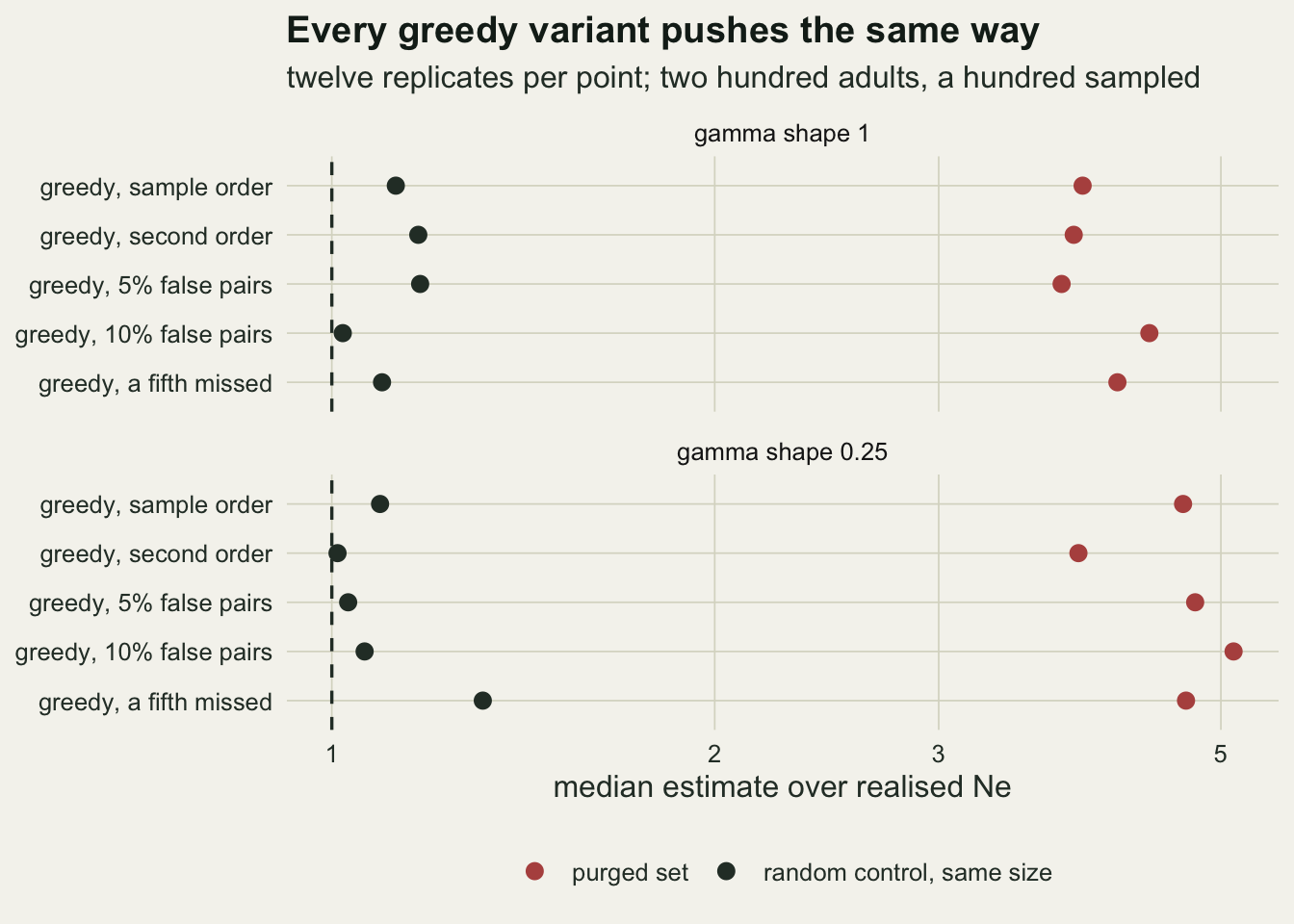
A sample built from families is a different problem
None of this contradicts the family sampling result. It completes it. Take the construction from the checking post: a fixed number of individuals collected as a few families of several offspring each, which is what a nest, a brood, a seed collection from a small number of mother trees or a single day at a spawning site delivers. The sample below is a hundred juveniles drawn as fifty families of two, twenty of five, or ten of ten, produced from the parental generation of the same simulated populations, with equal fecundity weights so that the population effective size is near the census.
make_kids <- function(hap_par, pa_vec, pb_vec, n_locus = 120) {
  n_kid <- length(pa_vec)
  pick <- function(par) {
    rows <- 2 * par - 1 + matrix(sample(0:1, n_kid * n_locus, TRUE),
                                 n_kid, n_locus)
    matrix(hap_par[cbind(as.vector(rows), rep(seq_len(n_locus), each = n_kid))],
           n_kid, n_locus)
  }
  kid <- matrix(0L, 2 * n_kid, n_locus)
  kid[seq(1, 2 * n_kid, 2), ] <- pick(pa_vec)
  kid[seq(2, 2 * n_kid, 2), ] <- pick(pb_vec)
  kid
}
sub_hap <- function(hap, idx) hap[as.vector(rbind(2 * idx - 1, 2 * idx)), ,
                                  drop = FALSE]

set.seed(73310)
n_nest <- 100
nest_rows <- NULL
for (r in 1:12) {
  pop <- sim_pop(200, Inf)
  for (per_fam in c(2, 5, 10)) {
    n_fam <- n_nest / per_fam
    sire  <- sample(200, n_fam)
    dam   <- sample(setdiff(seq_len(200), sire), n_fam)
    nest  <- make_kids(pop$hap_par, rep(sire, each = per_fam),
                       rep(dam, each = per_fam))
    one   <- seq(1, n_nest, by = per_fam)
    nest_rows <- rbind(nest_rows, data.frame(
      rep_id = r, per_fam = per_fam, n_fam = n_fam,
      whole   = ld_ne(nest) / pop$ne_true,
      purged  = ld_ne(sub_hap(nest, one)) / pop$ne_true,
      control = ld_ne(sub_hap(nest, sample(n_nest, n_fam))) / pop$ne_true,
      random  = ld_ne(take(pop$hap, sample(200, n_fam))) / pop$ne_true))
  }
}
nest_med <- aggregate(cbind(whole, purged, control, random) ~ per_fam + n_fam,
                      data = nest_rows, FUN = med_fin)
nest_fail <- tapply(nest_rows$purged, nest_rows$per_fam, n_fail)
rand_fail <- tapply(nest_rows$random, nest_rows$per_fam, n_fail)
nest_inf  <- sum(vapply(nest_rows[, c("whole", "purged", "control", "random")],
                        n_fail, 1L))
nest_est  <- 4 * nrow(nest_rows)
push_lo   <- min(nest_med$purged); push_hi <- max(nest_med$purged)
nest2  <- nest_med[nest_med$per_fam == 2, ]
nest5  <- nest_med[nest_med$per_fam == 5, ]
nest10 <- nest_med[nest_med$per_fam == 10, ]
The whole nest sample behaves as the checking post says it does once the families are large enough to matter. Fifty families of two give a median ratio of 1.00, so a sample made of sibling pairs drawn from half the adults in the population is still right. Twenty families of five give 0.32 and ten families of ten give 0.15: the more concentrated the sample is in a few parents, the smaller the population looks.
Purging changes the sign of the error and overshoots. One individual per family leaves 50, 20 and 10 individuals, and over the replicates that returned a finite estimate the median ratios are 4.0, 4.7 and 3.8. The two smaller purged sets also fail outright: at 20 and 10 individuals the purged sample fell below the permutation floor in 3 and 5 of the twelve replicates and returned no estimate at all, which is the failure the strict rule of the previous section runs into at the same sample sizes. The size of the push does not track how wrong the sample was before it: it lies between 3.8 and 4.7 in all three, applied to a sample that was already right, to one that was about 3 times too low and to one that was about 7 times too low.
Two controls of the same final size say where the push comes from. A random subsample of the nest sample itself gives 0.96, 0.37 and 0.18: it keeps whatever sibling pairs it happens to draw, it tracks the whole nest sample down, and it never fails, at ten individuals as at fifty. A random sample of the same size drawn from the population rather than from the nests gives 1.06, 0.85 and 0.78, with 3 of the twelve failing at 10 individuals. Neither control goes anywhere near four. The overshoot is the conditioning on unshared parents, not the smaller sample.
That is the single sentence the whole post is about. The purge is not a correction that knows where the truth is. It is a fixed push in one direction, applied to whatever the sample happened to contain. In a nest sample it pushes up from a number that was too low and lands somewhere above the truth; in a randomly sampled cohort it pushes up from a number that was already right.
key <- as.character(nest_med$per_fam)
nest_long <- rbind(
  data.frame(per_fam = nest_med$per_fam, ratio = nest_med$purged,
             fails = as.integer(nest_fail[key]), what = "one per family"),
  data.frame(per_fam = nest_med$per_fam, ratio = nest_med$whole,
             fails = 0L, what = "whole nest sample"),
  data.frame(per_fam = nest_med$per_fam, ratio = nest_med$control,
             fails = 0L, what = "random subsample of the nest"),
  data.frame(per_fam = nest_med$per_fam, ratio = nest_med$random,
             fails = as.integer(rand_fail[key]),
             what = "random sample from the population"))
nest_long$what <- factor(nest_long$what,
                         levels = c("one per family", "whole nest sample",
                                    "random subsample of the nest",
                                    "random sample from the population"))

ggplot(nest_long, aes(per_fam, ratio, colour = what, group = what)) +
  geom_hline(yintercept = 1, linetype = "dashed", colour = te_body,
             linewidth = 0.6) +
  geom_line(aes(linetype = what), linewidth = 0.8) +
  geom_point(aes(shape = what), size = 2.6) +
  geom_text(data = nest_long[nest_long$fails > 0, ],
            aes(label = sprintf("%d of 12 gave no estimate", fails),
                vjust = ifelse(what == "one per family", -1.2, 2.0)),
            size = 3, show.legend = FALSE) +
  scale_x_continuous(breaks = c(2, 5, 10), limits = c(1.2, 12.4)) +
  scale_y_log10(expand = expansion(mult = c(0.06, 0.16))) +
  scale_colour_manual(values = c(te_rust, te_gold, te_gold, te_body),
                      name = NULL) +
  scale_linetype_manual(values = c("solid", "solid", "22", "22"), name = NULL) +
  scale_shape_manual(values = c(16, 16, 1, 2), name = NULL) +
  labs(x = "offspring per family in the sample",
       y = "median estimate over realised Ne",
       title = "The purge pushes up from wherever the sample started",
       subtitle = "equal fecundity weights, two hundred adults, twelve replicates; medians over the estimates that came back finite") +
  guides(colour = guide_legend(nrow = 2), linetype = guide_legend(nrow = 2),
         shape = guide_legend(nrow = 2)) +
  theme_datasheet() +
  theme(legend.position = "bottom", plot.subtitle = element_text(size = 9))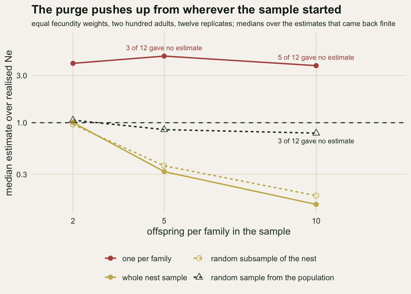
What to report
Say how the sample was collected before saying anything about relatedness. The two designs above need opposite treatment, and no property of the genotype file distinguishes them. A randomly sampled cohort needs no screening; a sample built from nests, broods or a handful of mother plants needs either a method that models the family structure or a different field season. The sampling protocol is the evidence, and it belongs in the methods paragraph next to the estimate.
If a purged estimate has to be reported, report the whole sample estimate beside it, and a random subsample of the purged size beside both. The third number is the one that settles the argument. In every cell of the grid above the random control sat within 40.5 per cent of the realised effective size, while the purged median sat 3.2 to 4.2 times higher than that control. Two numbers cannot tell those apart; three can.
Report the sibling pairs as a measurement. The mean shared parent count over the pairs of a random sample is four over the effective size, and the sibship frequency estimator of Wang is built on that relation. In this simulation, with the pedigree known, it recovered the realised effective size with a median ratio of 1.028. A program that has just spent an afternoon reconstructing families has produced an estimate of Ne, not a cleaning list.
Treat an estimate that rises when individuals are removed as a warning rather than an improvement. Removing individuals costs precision and cannot buy accuracy. If dropping half a sample raises the estimate threefold, that half was carrying the signal.
Honest limits
The purge here uses the true pedigree, with error added by hand. A sibship program infers families from the same genotypes that then go into the estimator, so its errors are correlated with the allele frequencies in a way that no addition or deletion of random pairs reproduces. The error arm shows that the inflation survives a pair list that is wrong in either direction at the rates tested; it does not show what a full reconstruction and estimation pipeline does on the same data, which would need the reconstruction itself.
The population is hermaphrodite with selfing allowed, which is the generator the rest of the effective size cluster uses. With separate sexes the half sibling structure differs: maternal and paternal half sibs arise at different rates when the sex ratio is uneven, and a purge that removes anything sharing either parent removes a different set. The direction of the effect follows from the shared parent identity, which does not depend on the mating system, but the magnitudes in the grid are for this generator.
The nest arm builds its families from disjoint sets of sires and dams, so the sampled families share no parents with each other and one individual per family is guaranteed to be a set with no shared parent in it at all. Real nests taken from a small adult pool do share parents, at a rate near one over the effective size, so the purged sets there are the most completely conditioned version of the rule available and the push they show is the largest the design can produce.
The truth is a choice. The linkage disequilibrium signal is dominated by the most recent parents, so the harmonic mean over six generations used here could reasonably be replaced by the single parental generation value. It makes no difference in this simulation, because the population is of constant size and the family size variance is redrawn independently every generation: the two versions of the truth have a median ratio of 0.997, and the purged median ratio moves from 3.97 to 3.93. In a population whose size is changing they would differ, and which window an estimate covers is the first of the checks in the post this one answers.
The loci are unlinked and neutral, the population is closed and of constant size, and generations are discrete. Every one of those assumptions is examined elsewhere in this cluster and each one moves the estimate on its own; none of them is being tested here, and the ratios above are ratios to the realised effective size of the same simulated population, not to a census.
Twelve replicates per cell is enough to place a median ratio near four against a control near one, and not enough to resolve a twenty per cent difference between two purge rules. The rule comparison should be read as a statement that the differences between rules are small against the effect, not as a measurement of those differences. The paired sign of the effect is what the design measures sharply: no exception in 139 paired draws puts the rate of exceptions below 0.021 with 95 per cent confidence.
The estimator returns an infinite value whenever the observed mean squared correlation falls below the permutation floor, and the three sets of runs above meet it at very different rates. It happened 5 times in the 432 whole sample, purged and control estimates of the grid, all 5 of them in purged sets; 13 times in the 288 estimates of the rule sweep, 12 of those in the strict one per group rule; and 11 times in the 144 estimates of the nest arm, entirely in the purged sets of 20 and 10 and in the population sample of 10. Taking medians over the finite estimates keeps those failures out of the numbers but not out of the account of them. A median over the estimates that came back is itself a selected quantity, and in the purged sets the selection runs one way: the estimates that did not come back are the samples whose correlation fell below their own floor, which is the far end of the same push, so the medians printed above are its low side and not a cleaned up version of it. The rate rises with the purge and with the smallness of what it leaves, so a single study that purges down to a few dozen individuals is in the regime where the estimator stops answering. Means would be worse than medians here, and a study with one sample and no replication has no way to know which side of the floor it is on. That failure mode is the subject of the estimation post, and nothing here repairs it.
References
Waples RS, Anderson EC 2017 Molecular Ecology 26(5):1211-1224 (10.1111/mec.14022)
Wang J 2009 Molecular Ecology 18(10):2148-2164 (10.1111/j.1365-294X.2009.04175.x)
Waples RS, Do C 2010 Evolutionary Applications 3(3):244-262 (10.1111/j.1752-4571.2009.00104.x)
Waples RS 2006 Conservation Genetics 7(2):167-184 (10.1007/s10592-005-9100-y)
Hill WG 1981 Genetical Research 38(3):209-216 (10.1017/S0016672300020553)
Crow JF, Kimura M 1970 An Introduction to Population Genetics Theory (ISBN 978-1932846126)