library(ggplot2)
library(patchwork)

te_paper  <- "#f5f4ee"
te_ink    <- "#16241d"
te_body   <- "#2c3a31"
te_forest <- "#275139"
te_rust   <- "#b5534e"
te_gold   <- "#c9b458"
te_line   <- "#dad9ca"
te_grey   <- "#8a948c"

theme_datasheet <- function() {
  theme_minimal(base_size = 12) +
    theme(plot.background  = element_rect(fill = te_paper, colour = NA),
          panel.background = element_rect(fill = te_paper, colour = NA),
          panel.grid.major = element_line(colour = te_line, linewidth = 0.3),
          panel.grid.minor = element_blank(),
          text             = element_text(colour = te_body),
          plot.title       = element_text(colour = te_ink, face = "bold"),
          plot.subtitle    = element_text(colour = te_body),
          axis.text        = element_text(colour = te_body))
}Sampling until the standard error is small
R
sampling design
count data
stopping rules
simulation
ecology tutorial
Counting quadrats until the running standard error is a quarter of the mean misses that precision. In R: the cost of a variable sample, and Green’s stop line.
A crew is counting snails in quarter metre quadrats along a lake shore, or ticks on a cloth dragged over ten metres of grass, or aphids on tillers in a wheat field. The protocol says to keep going until the standard error is a quarter of the mean, and never to stop before five units. After each quadrat someone works out the mean and the standard deviation of the counts so far, divides the standard error by the mean, and the crew moves on to the next site as soon as the ratio is 0.25 or less. On a site where the first quadrats happen to agree, the crew is done early. On a site where they disagree, it keeps counting. The rule is sensible and easy, and it promises a relative standard error of 0.25 at every site.
This post measures whether it keeps that promise. The comparison is against two older answers from insect sampling. Karandinos (1976) fixed the number of quadrats in advance from Taylor’s power law, and Green (1970) drew a stop line on the running total of insects, which reads the Taylor law instead of the sample variance. Kuno (1969) had built the same kind of line from Iwao’s regression of mean crowding on the mean a year earlier; Binns and Nyrop (1992) review these plans together with the classification plans used for spray decisions. On the statistical side, Chow and Robbins (1965) proved that a stop run on the sample variance reaches its nominal coverage and its ideal sample size only in the limit as the required width goes to zero. Their theorem concerns an interval of fixed absolute width, and it says nothing about how far off the rule is at the precision a field crew actually asks for. No source was found that reports the running rule’s shortfall at a relative standard error of 0.25, so this post measures it.
Several posts on this site sit next to this one. Sequential sampling for pest decisions simulates Wald’s classification plan only, and its honest limits list Green’s fixed precision stop lines among the plans that were not tested. Taylor’s power law and how many quadrats derives the fixed number of quadrats, Karandinos’ formula, and shows that the fitted exponent moves with the quadrat size. This post runs the informal running rule and Green’s line side by side with that fixed plan. The findings: at means of two per quadrat and above, most of the running rule’s loss is the price of a variable sample size, which is arithmetic once the stopping sizes are known; in sparse counts the rule’s reading of the mean adds about as much again; and Green’s line keeps its promise, to within a few per cent, only while its exponent is right.
Three more posts cover the same family of problems from other angles. Testing a monitoring series every year stops a series at the first significant trend test and notes that “Stopping at the first significant look is a selection rule, and it selects for extreme estimates”. There the stop reads an estimate; here it reads a precision estimate, and the mean it stops on leans high, most in sparse counts, rather than being extreme. Adaptive second-phase tows and the low mean lets a variance estimate move trawl tows between strata, and removal passes until the catch drops ends electrofishing passes on a ratio of catches. Standard errors and confidence intervals in R checks interval coverage by simulation at a fixed sample size, which is the yardstick the coverage column below is read against.
Three ways to decide how many quadrats
The counts follow Taylor’s power law: at a site with mean count m per quadrat the variance is a m^b. The generator draws negative binomial counts with that variance, and Poisson counts where the law would ask for less variance than the Poisson. The intercept a is 2 throughout, the exponent b is 1.5 or 1.8, and the mean is 0.5, 2 or 10 per quadrat, which spans a sparse benthic sample to a dense aphid count. All of these were fixed before anything ran.
Three plans aim at the same target, a relative standard error D of the mean. The fixed plan takes Karandinos’ number of quadrats, n* = a m^(b - 2) / D^2, rounded up. It needs the true mean, which no crew has; it is here as the plan that the other two are trying to imitate. The running rule computes s / (xbar sqrt(n)) after every quadrat from the minimum onwards and stops at the first value at or below D. Green’s line stops the first time the running total T_n reaches
T_n >= (D^2 / a)^(1 / (b - 2)) * n^((b - 1) / (b - 2))
and that line is not a separate idea. Replace the sample variance in the running rule by the variance the Taylor law predicts at the running mean, a xbar^b, and the condition sqrt(a xbar^b / n) <= D xbar rearranges into exactly this inequality once xbar = T_n / n is substituted; the direction flips because b - 2 is negative. So Green’s line is the running rule with the sample variance taken out. It reads the running mean and nothing else. The chunk checks that equivalence on a grid rather than asserting it.
a_tay   <- 2
m_set   <- c(0.5, 2, 10)
b_set   <- c(1.5, 1.8)
D_main  <- 0.25
D_fine  <- 0.1
min_set <- c(5, 10)
b_shift <- 0.2
n_field <- 1000
K_reg   <- 50

rcount <- function(n, m, a, b) {
  v_pow <- a * m^b
  if (v_pow <= m) return(rpois(n, m))
  rnbinom(n, mu = m, size = m^2 / (v_pow - m))
}

n_star_of <- function(m, b, D) a_tay * m^(b - 2) / D^2

green_line <- function(n, D, a, b) (D^2 / a)^(1 / (b - 2)) * n^((b - 1) / (b - 2))

check_grid <- expand.grid(n = 5:80, tot = 1:400, b = b_set)
check_grid <- check_grid[abs(sqrt(a_tay * (check_grid$tot / check_grid$n)^check_grid$b /
  check_grid$n) / (check_grid$tot / check_grid$n) - D_main) > 1e-9, ]
by_taylor <- with(check_grid,
  sqrt(a_tay * (tot / n)^b / n) <= D_main * tot / n)
by_line   <- with(check_grid, tot >= green_line(n, D_main, a_tay, b))
n_agree   <- sum(by_taylor == by_line)

cells <- expand.grid(m = m_set, b = b_set)
cells$n_star <- ceiling(n_star_of(cells$m, cells$b, D_main))
cells
m b n_star
1 0.5 1.5 46
2 2.0 1.5 23
3 10.0 1.5 11
4 0.5 1.8 37
5 2.0 1.8 28
6 10.0 1.8 21The two forms of Green’s condition agree on 60794 of 60794 combinations of quadrat number and running total, which is all of them. At D of 0.25 the fixed plan asks for 46, 23, 11, 37, 28, 21 quadrats in the six cells of the table, from 11 for dense counts with the lower exponent to 46 for the sparsest.
A thousand sites per batch
Each batch draws the counts of 1000 sites in one cell, as a matrix with one row per site and enough columns that no rule runs out of quadrats, then reads every plan off the same rows. Every arm in a batch therefore sees the same counts, and differences between arms are not differences between random draws. The running sums of the counts and of their squares give the mean and the standard error after every quadrat in two passes over the columns.
Two plans are there only as yardsticks. A fixed plan with the running rule’s own average number of quadrats, rounded, is the fair comparator on cost: it spends the same effort as the rule on average, so any gap between the two is the cost of letting the number vary. Like Karandinos’ plan, it is set for the one density of its cell, which a crew would have to know in advance. The second yardstick is a thought experiment. It stops on s / (m sqrt(n)) <= D with the true mean m in the denominator, which no crew can compute; it isolates the half of the running rule that reads the variance. A last arm gives Green’s line an exponent 0.2 lower than the truth, with a unchanged. That error is well inside the range of exponents the Taylor post finds when the same fields are counted with quadrats of different sizes.
first_hit <- function(ok, n_max) {
  k <- max.col(ok, "first")
  k[rowSums(ok) == 0] <- n_max
  k
}

sim_block <- function(m, b, D, seed, keep_n = FALSE) {
  set.seed(seed)
  n_star <- ceiling(n_star_of(m, b, D))
  n_max  <- max(4 * n_star, 60)
  x_mat  <- matrix(rcount(n_field * n_max, m, a_tay, b), n_field, n_max)
  s_one  <- x_mat
  s_two  <- x_mat^2
  for (j in 2:n_max) {
    s_one[, j] <- s_one[, j - 1] + x_mat[, j]
    s_two[, j] <- s_two[, j - 1] + x_mat[, j]^2
  }
  nn     <- matrix(seq_len(n_max), n_field, n_max, byrow = TRUE)
  x_bar  <- s_one / nn
  se_run <- sqrt(pmax((s_two - nn * x_bar^2) / pmax(nn - 1, 1), 0) / nn)
  row_id <- seq_len(n_field)
  reg_id <- rep(seq_len(n_field / K_reg), each = K_reg)
  score <- function(arm, n_min, k) {
    est  <- x_bar[cbind(row_id, k)]
    se_k <- se_run[cbind(row_id, k)]
    tot  <- s_one[cbind(row_id, k)]
    r_tot <- rowsum(tot, reg_id)[, 1] / rowsum(k, reg_id)[, 1]
    r_msm <- rowsum(est, reg_id)[, 1] / K_reg
    data.frame(m = m, b = b, D = D, n_min = n_min, seed = seed, arm = arm,
               n_star = n_star, n_star_exact = n_star_of(m, b, D),
               sum_est = sum(est), sum_sq = sum(est^2),
               inv_n = mean(1 / k), mean_n = mean(k),
               p_short = mean(k <= n_star / 2),
               cover = mean(abs(est - m) <= qt(0.975, pmax(k - 1, 1)) * se_k),
               hit_max = mean(k == n_max),
               sum_dev2 = sum((tot - m * k)^2),
               sum_rt = sum(r_tot), sq_rt = sum(r_tot^2),
               sum_rm = sum(r_msm), sq_rm = sum(r_msm^2))
  }
  out  <- list()
  kept <- NULL
  for (n_min in min_set) {
    k_rule <- first_hit((nn >= n_min) & (x_bar > 0) & (se_run <= D * x_bar), n_max)
    k_grn  <- first_hit((nn >= n_min) & (s_one >= green_line(nn, D, a_tay, b)), n_max)
    k_gmis <- first_hit((nn >= n_min) &
                        (s_one >= green_line(nn, D, a_tay, b - b_shift)), n_max)
    n_eq   <- round(mean(k_rule))
    out[[length(out) + 1]] <- rbind(
      score("running rule", n_min, k_rule),
      score("fixed at the rule's mean N", n_min, rep(n_eq, n_field)),
      score("fixed n*", n_min, rep(n_star, n_field)),
      score("Green, true b", n_min, k_grn),
      score("Green, b - 0.2", n_min, k_gmis))
    if (n_min == min(min_set) && D == D_main) {
      k_orc <- first_hit((nn >= n_min) & (se_run <= D * m), n_max)
      out[[length(out) + 1]] <- score("variance only", n_min, k_orc)
    }
    if (keep_n && n_min == min(min_set)) kept <- data.frame(
      N = c(k_rule, k_grn),
      arm = rep(c("running rule", "Green, true b"), each = n_field))
  }
  list(summary = do.call(rbind, out), kept = kept)
}
The batches run at two precisions. At D of 0.25 each cell gets twenty batches, twenty thousand sites; at D of 0.1, where the sites need up to a few hundred quadrats each and the matrices are much larger, ten batches. The batch counts were fixed before the run. Batches double as the Monte Carlo yardstick: every ratio below carries a standard error taken from the spread of its batch values.
n_batch_main <- 20
n_batch_fine <- 10
keep_m <- 2
keep_b <- 1.5
blocks <- list()
kept_n <- NULL
for (i in seq_len(nrow(cells))) {
  for (s in seq_len(n_batch_main)) {
    keep <- cells$m[i] == keep_m && cells$b[i] == keep_b && s == 1
    rb <- sim_block(cells$m[i], cells$b[i], D_main, 1000 * i + s, keep_n = keep)
    blocks[[length(blocks) + 1]] <- rb$summary
    if (keep) kept_n <- rb$kept
  }
  for (s in seq_len(n_batch_fine)) {
    rb <- sim_block(cells$m[i], cells$b[i], D_fine, 50000 + 1000 * i + s)
    blocks[[length(blocks) + 1]] <- rb$summary
  }
}
batch_tab <- do.call(rbind, blocks)
batch_tab$cvr  <- sqrt((batch_tab$sum_sq - batch_tab$sum_est^2 / n_field) /
                       (n_field - 1)) / batch_tab$m / batch_tab$D
batch_tab$pred <- sqrt(batch_tab$n_star_exact * batch_tab$inv_n)
batch_tab$sel  <- batch_tab$cvr / batch_tab$pred
batch_tab$bias <- batch_tab$sum_est / n_field / batch_tab$m - 1

grp <- interaction(batch_tab$m, batch_tab$b, batch_tab$D, batch_tab$n_min,
                   batch_tab$arm, drop = TRUE)
pool_one <- function(z) {
  n_all <- n_field * nrow(z)
  mu    <- sum(z$sum_est) / n_all
  sd_all <- sqrt((sum(z$sum_sq) - n_all * mu^2) / (n_all - 1))
  inv_n <- mean(z$inv_n)
  n_reg <- n_all / K_reg
  reg_sd <- function(s1, s2) sqrt((sum(s2) - sum(s1)^2 / n_reg) / (n_reg - 1))
  data.frame(m = z$m[1], b = z$b[1], D = z$D[1], n_min = z$n_min[1], arm = z$arm[1],
             n_star = z$n_star[1], n_star_exact = z$n_star_exact[1],
             n_batch = nrow(z), cvr = sd_all / z$m[1] / z$D[1],
             cvr_se = sd(z$cvr) / sqrt(nrow(z)),
             pred = sqrt(z$n_star_exact[1] * inv_n),
             bias = mu / z$m[1] - 1, bias_se = sd(z$bias) / sqrt(nrow(z)),
             sel_se = sd(z$sel) / sqrt(nrow(z)),
             mean_n = mean(z$mean_n), inv_n = inv_n, p_short = mean(z$p_short),
             cover = mean(z$cover), hit_max = mean(z$hit_max),
             wald2 = sum(z$sum_dev2) / n_all / (a_tay * z$m[1]^z$b[1] * mean(z$mean_n)),
             n_reg = n_reg,
             reg_tot_bias = sum(z$sum_rt) / n_reg / z$m[1] - 1,
             reg_msm_bias = sum(z$sum_rm) / n_reg / z$m[1] - 1,
             reg_tot_sd = reg_sd(z$sum_rt, z$sq_rt),
             reg_msm_sd = reg_sd(z$sum_rm, z$sq_rm))
}
res <- do.call(rbind, lapply(split(batch_tab, grp), pool_one))
res$sel <- res$cvr / res$pred
res <- res[order(res$D, res$n_min, res$arm, res$b, res$m), ]
rownames(res) <- NULL
pick <- function(arm, D = D_main, n_min = 5) {
  z <- res[res$arm == arm & res$D == D & res$n_min == n_min, ]
  z[order(z$b, z$m), ]
}
rule  <- pick("running rule")
feq   <- pick("fixed at the rule's mean N")
fstar <- pick("fixed n*")
grn   <- pick("Green, true b")
gmis  <- pick("Green, b - 0.2")
orc   <- pick("variance only")
hit_any <- max(res$hit_max)
The running rule misses its promise
The measure of precision is the one the rule promises. For each cell, take the spread of the stopped means across all the sites, divide by the true mean, and divide again by the promised D. A ratio of one means the plan delivered exactly what it promised; 1.2 means its means are 20 per cent noisier than promised. This is a ratio over sites, and each site contributes one stopped mean. No site in any arm ran out of quadrats (the largest share that hit the cap was 0.000).
arm_levels <- c("running rule", "fixed at the rule's mean N", "fixed n*",
                "Green, true b", "Green, b - 0.2")
arm_cols <- c(te_rust, te_gold, te_forest, te_ink, te_grey)
plot_main <- res[res$D == D_main & res$n_min == 5 & res$arm %in% arm_levels, ]
plot_main$arm  <- factor(plot_main$arm, levels = arm_levels)
plot_main$m_f  <- factor(sprintf("m = %g", plot_main$m),
                         levels = sprintf("m = %g", m_set))
plot_main$b_f  <- sprintf("b = %.1f", plot_main$b)
dodge <- position_dodge(width = 0.75)

p_promise <- ggplot(plot_main, aes(m_f, cvr, colour = arm)) +
  geom_hline(yintercept = 1, linetype = "dashed", colour = te_body, linewidth = 0.5) +
  geom_point(aes(y = pred), shape = 21, fill = te_paper, size = 3.2,
             stroke = 0.9, position = dodge) +
  geom_point(size = 2.4, position = dodge) +
  facet_wrap(~ b_f) +
  scale_colour_manual(values = arm_cols, name = NULL) +
  labs(x = "mean count per quadrat",
       y = "achieved relative SE / promised",
       title = "The running rule is noisier than it promises",
       subtitle = "filled: achieved; hollow: predicted from the stopping sizes; D = 0.25, minimum 5") +
  theme_datasheet() +
  theme(legend.position = "bottom") +
  guides(colour = guide_legend(nrow = 2))
p_promise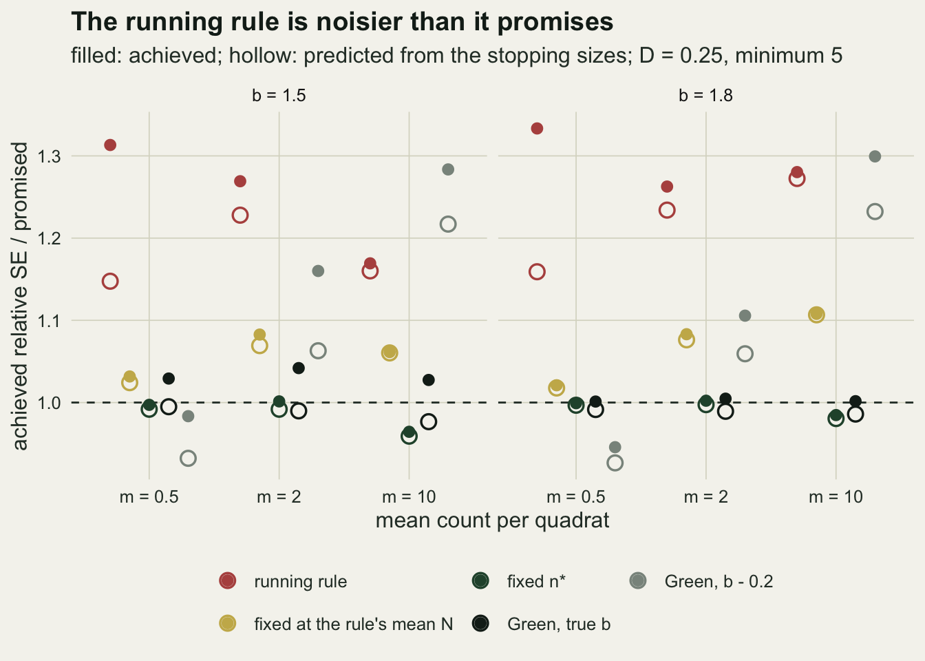
The running rule delivers a ratio of 1.17 to 1.33 across the six cells, with Monte Carlo standard errors of at most 0.020. The fixed plan at Karandinos’ n* delivers 0.96 to 1.00; its lowest value is in the dense cell with b of 1.5, where rounding 10.12 up to 11 quadrats buys a little more precision than was asked for. Green’s line with the true constants delivers 1.00 to 1.04.
The rule also stops earlier than the fixed plan on average: 8.9 quadrats against 11 in the dense cell with the lower exponent, and between 4 and 22 per cent fewer quadrats across the cells. That is part of the story and not most of it. The fair comparison is the gold arm: a fixed plan that spends the rule’s own average effort at the known density of the cell. Against it, the running rule’s ratio is 1.10 to 1.31 times larger, with a median over the six cells of 1.169. Where the density is known, spending the same number of quadrats on every site, instead of letting the counts decide, buys that much precision for nothing.
The miss is mostly arithmetic on N, except in sparse counts
Why a variable number of quadrats costs precision has a two-line answer. Suppose for a moment that the stopping size N were drawn independently of the counts. Given N = n, the mean of n counts has variance a m^b / n, and its expectation is m whatever n is, so the variance of the stopped mean is a m^b E[1/N]. Divided by m^2 and by D^2, the ratio plotted above would be
sqrt(n*exact E[1/N]) = sqrt(n*exact / E[N]) * sqrt(E[N] E[1/N])
where n*exact is Karandinos’ number before rounding. The first factor is the price of fewer quadrats on average. The second is at least one for any N that varies, because 1/N is convex (Jensen’s inequality), and it equals one only when every site gets the same number. A site that stops at five quadrats loses more precision than a site that goes on to fifteen gains back. None of this is a finding: it is closed form once the distribution of N is known, and the hollow points in the figure are this prediction computed from each arm’s own stopping sizes. What the simulation adds is the distribution of N, and a check of whether the independence assumption holds.
kept_n$arm <- factor(kept_n$arm, levels = c("running rule", "Green, true b"))
keep_star  <- cells$n_star[cells$m == keep_m & cells$b == keep_b]
n_short_rule <- mean(kept_n$N[kept_n$arm == "running rule"] <= keep_star / 2)
n_min_rule   <- mean(kept_n$N[kept_n$arm == "running rule"] == min(min_set))
sd_n_rule    <- sd(kept_n$N[kept_n$arm == "running rule"])
sd_n_green   <- sd(kept_n$N[kept_n$arm == "Green, true b"])
range_green <- range(kept_n$N[kept_n$arm == "Green, true b"])ggplot(kept_n, aes(N)) +
geom_histogram(binwidth = 1, fill = te_forest, colour = te_paper, linewidth = 0.2) +
geom_vline(xintercept = keep_star, linetype = "dashed", colour = te_ink,
linewidth = 0.6) +
geom_vline(xintercept = keep_star / 2, linetype = "dotted", colour = te_rust,
linewidth = 0.8) +
facet_wrap(~ arm, ncol = 1) +
labs(x = "quadrats counted before stopping", y = "sites",
title = "The running rule stops early at many sites",
subtitle = sprintf("dashed: n* = %d; dotted red: n*/2; one batch of %d sites",
keep_star, n_field)) +
theme_datasheet()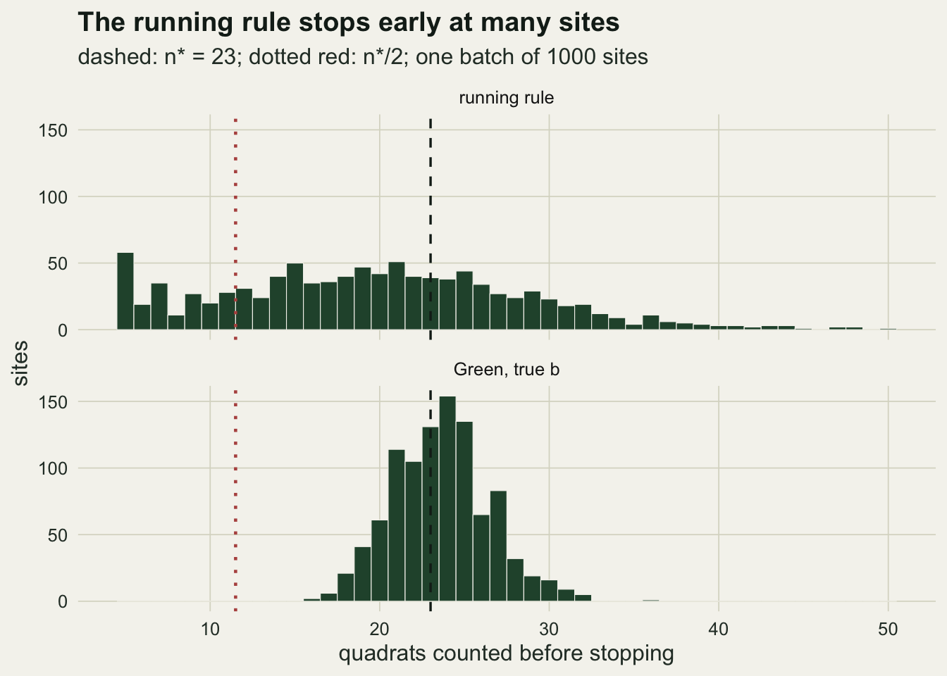
In this cell, with a mean of 2 per quadrat and b of 1.5, the fixed plan wants 23 quadrats. Under the running rule 19.8 per cent of the sites stopped at half that or fewer, and 5.8 per cent stopped at the minimum of five. The standard deviation of the stopping size is 8.8 quadrats under the running rule and 2.9 under Green’s line, which stopped every site between 16 and 36 quadrats. Across all six cells the share of sites stopping at or below half of n* under the running rule is 9.1 to 27.2 per cent, highest where n* is smallest.
The short tail is what the rule buys. When the first few counts happen to be similar, the sample standard deviation is small, the ratio clears 0.25 early, and the site is left with a mean of five or six counts. The table puts the three factors side by side for the running rule, with the achieved ratio beside the prediction.
dec_tab <- data.frame(
  m = rule$m, b = rule$b,
  mean_N = round(rule$mean_n, 1),
  effort = round(sqrt(rule$n_star_exact / rule$mean_n), 3),
  spread = round(sqrt(rule$mean_n * rule$inv_n), 3),
  predicted = round(rule$pred, 3),
  achieved = round(rule$cvr, 3),
  selection = round(rule$sel, 3),
  sel_se = round(rule$sel_se, 3))
dec_tab
m b mean_N effort spread predicted achieved selection sel_se
1 0.5 1.5 43.1 1.025 1.120 1.148 1.313 1.144 0.015
2 2.0 1.5 19.7 1.071 1.146 1.228 1.269 1.034 0.010
3 10.0 1.5 8.9 1.065 1.089 1.160 1.169 1.008 0.007
4 0.5 1.8 35.5 1.018 1.138 1.159 1.333 1.150 0.009
5 2.0 1.8 24.1 1.075 1.148 1.234 1.263 1.023 0.007
6 10.0 1.8 16.5 1.108 1.149 1.273 1.280 1.006 0.007spread_rng <- range(sqrt(rule$mean_n * rule$inv_n))
effort_rng <- range(sqrt(rule$n_star_exact / rule$mean_n))
sel_dense <- rule[rule$m >= 2, ]
sel_sparse <- rule[rule$m < 1, ]
feq_gap <- max(abs(feq$sel - 1))
n_spread_big <- sum(sqrt(rule$mean_n * rule$inv_n) > sqrt(rule$n_star_exact / rule$mean_n))
z_two <- (sel_dense$sel[sel_dense$m == 2] - 1) / sel_dense$sel_se[sel_dense$m == 2]The spread factor, the Jensen term, is 1.089 to 1.149, and the effort factor 1.018 to 1.108. The spread of N is the larger of the two in 6 of the 6 cells. The last two columns test the independence assumption. At a mean of 10 per quadrat the achieved ratio sits on the prediction (selection factors of 1.008 and 1.006, standard errors about 0.007). At a mean of 2 the achieved ratio is 1.034 and 1.023 times the prediction, a small excess, but 3.5 and 3.3 standard errors from one. At a mean of 0.5 it is 1.144 and 1.150 times the prediction: in sparse counts the stopping size is not independent of the counts, and the next section shows why. As a control, the fixed plan at the rule’s mean N sits within 0.013 of its own prediction in every cell, which is what a sample size that does not read the data should do.
What the rule reads: the mean as well as the variance
The running rule’s ratio has the sample standard deviation on top and the sample mean underneath, and under a Taylor law with b below 2 the two move together. The thought experiment separates them. With the true mean in the denominator, the stop reads only the variance, and a site whose early counts are low has a low variance too, so it stops early on a low mean.
bias_arms <- c("variance only", "running rule", "Green, true b")
bias_df <- res[res$D == D_main & res$n_min == 5 & res$arm %in% bias_arms, ]
bias_df$arm  <- factor(bias_df$arm, levels = bias_arms)
bias_df$cell <- factor(sprintf("m %g, b %.1f", bias_df$m, bias_df$b),
                       levels = sprintf("m %g, b %.1f", cells$m, cells$b))
orc_out  <- sum(abs(orc$bias) > 0.05)
cov_rule <- range(rule$cover)
cov_feq  <- range(feq$cover)
cov_orc  <- range(orc$cover)
cov_loss <- max(feq$cover - rule$cover)ggplot(bias_df, aes(cell, bias, colour = arm)) +
geom_hline(yintercept = 0, linetype = "dashed", colour = te_body, linewidth = 0.5) +
geom_errorbar(aes(ymin = bias - 2 * bias_se, ymax = bias + 2 * bias_se),
width = 0.25, linewidth = 0.5, position = position_dodge(width = 0.6)) +
geom_point(size = 2.6, position = position_dodge(width = 0.6)) +
scale_colour_manual(values = c(te_grey, te_rust, te_ink), name = NULL,
labels = c("variance only (true mean, a thought experiment)",
"running rule", "Green, true b")) +
labs(x = NULL, y = "relative bias of the stopped mean",
title = "Dividing by the mean flips the sign",
subtitle = "D = 0.25, minimum 5 quadrats, 20000 sites per cell") +
theme_datasheet() +
theme(legend.position = "bottom", axis.text.x = element_text(size = 9)) +
guides(colour = guide_legend(nrow = 2))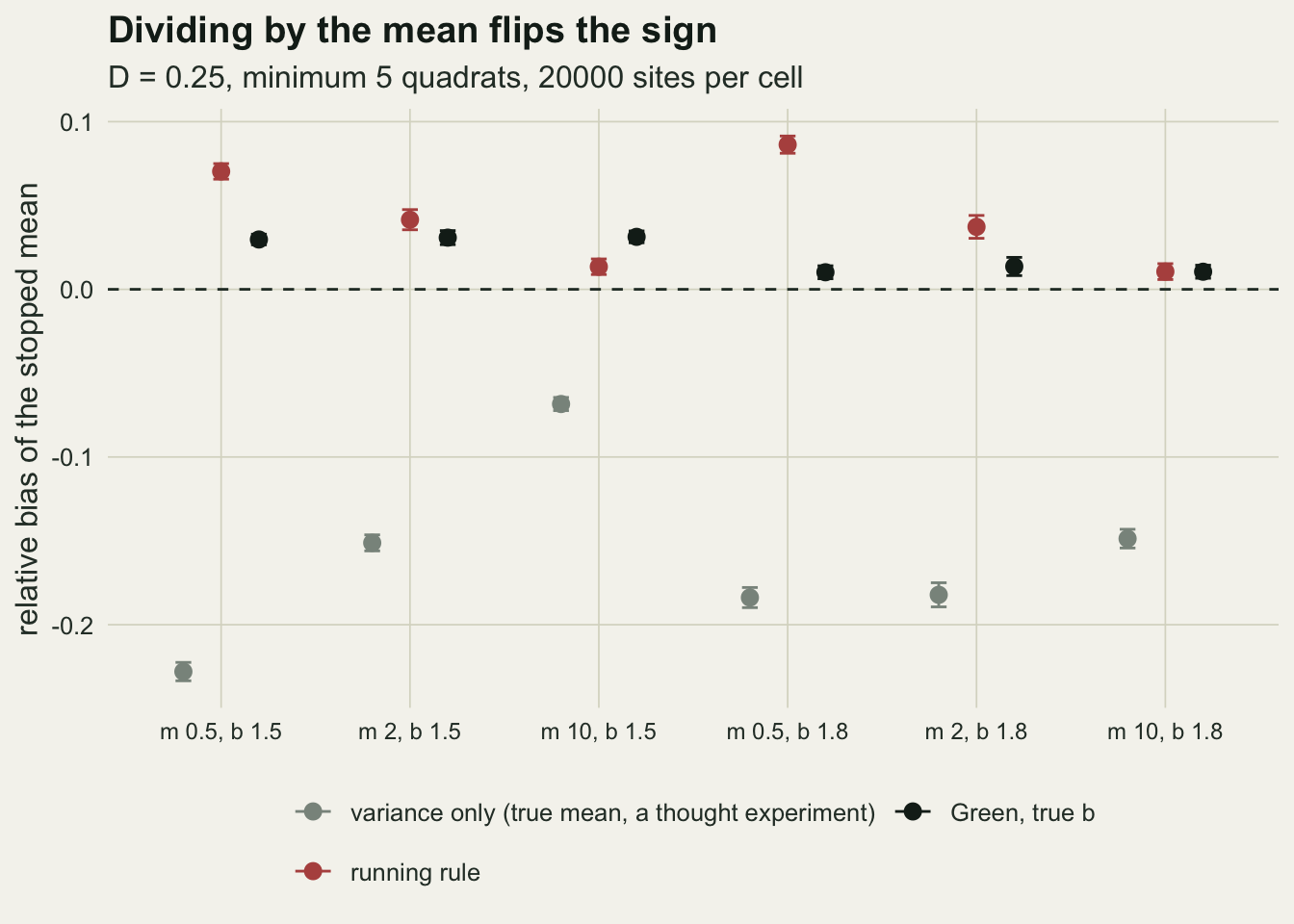
Stopping on the variance alone biases the mean low in every cell, by 6.8 to 22.8 per cent, and by more than five per cent in 6 of the 6 cells. This arm is not a plan anyone could run, since it needs the true mean; it exists to show which way the variance pulls. The running rule divides by the sample mean, and that cancels most of the pull: its bias is +0.011 to +0.086, and positive in every cell. The cancellation overshoots in sparse counts. At a mean of 0.5 a site whose first quadrats hold a few more animals than usual has a large xbar, a ratio that clears 0.25 early, and a stopped mean that is too high; the bias there is +0.070 and +0.086. That is the selection the previous table measured as the excess over the prediction, and it is not in the Jensen arithmetic. Green’s line reads only the running total, stops early when the total is high, and so leans high as well, by +0.010 to +0.031, the familiar lean of any plan that samples until a total is reached.
The coverage of the usual interval, xbar plus or minus t on n - 1 degrees of freedom times the standard error, is the secondary column. The running rule covers 0.891 to 0.943 against 0.908 to 0.933 for the fixed plan at the rule’s mean effort, so at most 1.8 points go missing against the fair comparator, and in the sparse cells the rule covers slightly better than the fixed plan. Neither reaches 0.95: the mean of 9 to 43 counts this skewed is itself skewed, and the standard errors post shows the same t interval slipping below 95 per cent with five skewed observations. Coverage is not where this rule’s cost shows. The variance-only thought experiment is different: it covers 0.740 to 0.907, because its low means come with low standard errors.
A larger minimum, a finer target, and a borrowed exponent
Two changes a crew could make, and one mistake it could make, are run on the same batches: a minimum of ten quadrats instead of five, a finer target of D equal to 0.1, and, for Green’s line, an exponent 0.2 too low.
rule_10  <- pick("running rule", D_main, 10)
feq_10   <- pick("fixed at the rule's mean N", D_main, 10)
rule_f5  <- pick("running rule", D_fine, 5)
feq_f5   <- pick("fixed at the rule's mean N", D_fine, 5)
rule_f10 <- pick("running rule", D_fine, 10)
gmis_f   <- pick("Green, b - 0.2", D_fine, 5)
grn_gap  <- max(grn$cvr - fstar$cvr)
grn_f    <- pick("Green, true b", D_fine, 5)
nstar_f  <- rule_f5$n_star

rep_df <- rbind(
  data.frame(rule[, c("m", "b", "cvr", "cvr_se")], setting = "D 0.25, minimum 5"),
  data.frame(rule_10[, c("m", "b", "cvr", "cvr_se")], setting = "D 0.25, minimum 10"),
  data.frame(rule_f5[, c("m", "b", "cvr", "cvr_se")], setting = "D 0.1, minimum 5"),
  data.frame(rule_f10[, c("m", "b", "cvr", "cvr_se")], setting = "D 0.1, minimum 10"))
gm_df <- rbind(
  data.frame(gmis[, c("m", "b", "cvr", "cvr_se")], setting = "D 0.25"),
  data.frame(gmis_f[, c("m", "b", "cvr", "cvr_se")], setting = "D 0.1"))
for (nm in c("rep_df", "gm_df")) {
  z <- get(nm)
  z$cell <- factor(sprintf("m %g, b %.1f", z$m, z$b),
                   levels = sprintf("m %g, b %.1f", cells$m, cells$b))
  assign(nm, z)
}
set_levels <- c("D 0.25, minimum 5", "D 0.25, minimum 10",
"D 0.1, minimum 5", "D 0.1, minimum 10")
rep_df$setting <- factor(rep_df$setting, levels = set_levels)
gm_df$setting <- factor(gm_df$setting, levels = c("D 0.25", "D 0.1"))
y_lim <- range(c(rep_df$cvr, gm_df$cvr, 0.9, 1))
p_rep <- ggplot(rep_df, aes(cell, cvr, colour = setting)) +
geom_hline(yintercept = 1, linetype = "dashed", colour = te_body, linewidth = 0.5) +
geom_point(size = 2.4, position = position_dodge(width = 0.6)) +
scale_colour_manual(values = c(te_rust, te_gold, te_forest, te_ink), name = NULL) +
scale_y_continuous(limits = y_lim) +
labs(x = NULL, y = "achieved / promised",
title = "A. Running rule") +
theme_datasheet() +
theme(legend.position = "bottom", axis.text.x = element_text(size = 8,
angle = 30, hjust = 1)) +
guides(colour = guide_legend(nrow = 2))
p_gm <- ggplot(gm_df, aes(cell, cvr, colour = setting)) +
geom_hline(yintercept = 1, linetype = "dashed", colour = te_body, linewidth = 0.5) +
geom_point(size = 2.4, position = position_dodge(width = 0.5)) +
scale_colour_manual(values = c(te_rust, te_forest), name = NULL) +
scale_y_continuous(limits = y_lim) +
labs(x = NULL, y = NULL, title = "B. Green, b - 0.2") +
theme_datasheet() +
theme(legend.position = "bottom", axis.text.x = element_text(size = 8,
angle = 30, hjust = 1))
(p_rep | p_gm) + plot_layout(widths = c(1.3, 1)) +
plot_annotation(theme = theme_datasheet())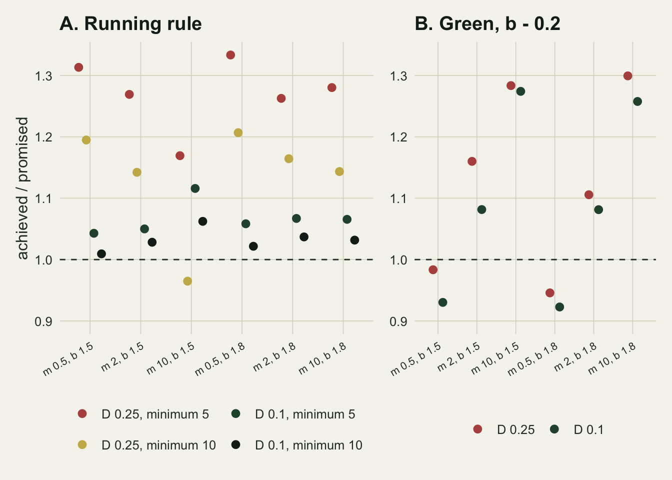
A minimum of ten quadrats is a partial repair. The running rule’s ratio drops to 0.96 to 1.21, and its excess over the fixed plan at the same mean effort to 1.02 to 1.19 times. The repair works best in the dense cell with the lower exponent, where n* is 11 and a minimum of ten leaves the rule with almost nothing to decide.
A finer target is the Chow and Robbins direction, and it holds here. At D of 0.1 the fixed plan wants 64 to 283 quadrats, the short tail becomes rare (3.9 per cent of sites at half of n* or below at worst), and the running rule’s ratio falls to 1.04 to 1.12 with a minimum of five, with Monte Carlo standard errors up to 0.015 from its ten batches. The rule’s cost is a small-sample cost, and asking for more precision shrinks it along with the samples.
Green’s line with the true constants stays at 0.99 to 1.01 at D of 0.1. What happens with its exponent 0.2 too low can be worked out before any simulation. The line with exponent b' = b - 0.2 is the running rule with a xbar^b' in place of the sample variance, so it stops near Karandinos’ number for the wrong exponent, n*' = a m^(b' - 2) / D^2 = n* m^(-0.2) quadrats. The counts still have variance a m^b, so the relative standard error at that size is sqrt(a m^(b - 2) / n*') = D m^0.1. The line misses its promise by a factor of about m^0.1: 0.933, 1.072, 1.259 at means of 0.5, 2 and 10. The factor holds no D, so a finer target cannot remove it, and it moves with the mean: an exponent that is too low predicts too little variance above a mean of one and too much below it. The chunk sets the algebra beside the simulation: the se_ columns give the ratio of the misspecified line’s achieved value to that of the line with the true exponent, and the N_ columns the same ratio for the average number of quadrats, against m^(-0.2).
shift_pred <- gmis$m^(b_shift / 2)
shift_tab <- data.frame(
  m = gmis$m, b = gmis$b,
  se_pred = round(shift_pred, 3),
  se_D0.25 = round(gmis$cvr / grn$cvr, 3),
  se_D0.1 = round(gmis_f$cvr / grn_f$cvr, 3),
  N_pred = round(gmis$m^(-b_shift), 3),
  N_D0.1 = round(gmis_f$mean_n / grn_f$mean_n, 3))
shift_tab
m b se_pred se_D0.25 se_D0.1 N_pred N_D0.1
1 0.5 1.5 0.933 0.956 0.939 1.149 1.149
2 2.0 1.5 1.072 1.113 1.079 0.871 0.872
3 10.0 1.5 1.259 1.249 1.263 0.631 0.636
4 0.5 1.8 0.933 0.945 0.934 1.149 1.149
5 2.0 1.8 1.072 1.100 1.075 0.871 0.872
6 10.0 1.8 1.259 1.297 1.262 0.631 0.633shift_dev_fine <- max(abs(gmis_f$cvr / grn_f$cvr - shift_pred))
shift_dev_main <- max(abs(gmis$cvr / grn$cvr - shift_pred))
g10 <- gmis[gmis$m == 10, ]
r10 <- rule[rule$m == 10, ]
gap_z <- sapply(b_set, function(bb) {
in_cell <- batch_tab$D == D_main & batch_tab$n_min == 5 & batch_tab$m == 10 &
batch_tab$b == bb
d <- batch_tab$cvr[in_cell & batch_tab$arm == "Green, b - 0.2"] -
batch_tab$cvr[in_cell & batch_tab$arm == "running rule"]
mean(d) / (sd(d) / sqrt(length(d)))
})At D of 0.1 the simulated ratio is within 0.008 of m^0.1 in every cell, and at D of 0.25, where the stopping sizes are small and the approximation coarser, within 0.042. Set against the running rule at D of 0.25, the misspecified line delivers 1.11 to 1.30 at means of 2 and 10, against 1.17 to 1.28 for the rule. It is better than the rule at a mean of 2 and worse at 10, where it delivers 1.28 against 1.17 with b of 1.5, and 1.30 against 1.28 with b of 1.8, gaps of 23 and 2.2 standard errors of the batch-by-batch difference. At D of 0.1 it is still 1.08 to 1.27 there, while the running rule’s ratio falls as the target tightens. Below a mean of one the line overshoots, which is safe and wasteful: 53.5 quadrats against 46 in the sparse cell with b of 1.5, and a ratio of 0.98.
Many sites pooled into one mean
Everything so far is the precision of the mean at one site. A survey that pools many sites into a regional mean can do it in two ways, and they behave differently. The mean of the site means is an average of stopped means, so it keeps each site’s bias, and its spread relative to the same average under the fixed plan is the site-level ratio again. The total count over all sites divided by the total number of quadrats keeps neither, and that is closed form too. Wald’s identity says that for any rule that decides after each quadrat on the counts so far, the expected running total at the stop is m E[N], so when the sites share one density the ratio of the two totals settles on m as sites are added. Wald’s second identity says that E[(T_N - m N)^2] = a m^b E[N], which makes the variance of that ratio over K sites about a m^b / (K E[N]): the variance of a fixed plan with the same number of quadrats in total. Once many sites are summed, the variable N stops mattering. That holds only while the sites share one density, as every cell here does. Where densities differ, the same identity applied site by site says that the ratio of totals settles on the site densities averaged with each site’s expected number of quadrats as its weight, and the running rule counts the most quadrats where counts are sparsest (43.1 at a mean of 0.5 against 8.9 at 10 with b of 1.5), so the ratio of totals leans towards the sparse sites and no longer estimates the mean site density. The chunk groups each batch of a thousand sites into regions of 50 and checks both estimators against the fixed plan at the rule’s mean N, grouped the same way; the means_ columns are the mean of the site means and the totals_ columns the ratio of totals, with each spread given as a multiple of the fixed plan’s.
pool_tab <- data.frame(
  m = rule$m, b = rule$b,
  means_bias = round(rule$reg_msm_bias, 3),
  totals_bias = round(rule$reg_tot_bias, 3),
  means_sd = round(rule$reg_msm_sd / feq$reg_msm_sd, 3),
  totals_sd = round(rule$reg_tot_sd / feq$reg_msm_sd, 3),
  wald_two = round(rule$wald2, 3))
pool_tab
m b means_bias totals_bias means_sd totals_sd wald_two
1 0.5 1.5 0.070 -0.002 1.269 1.011 1.001
2 2.0 1.5 0.042 0.002 1.183 1.007 1.018
3 10.0 1.5 0.013 0.004 1.089 1.014 1.021
4 0.5 1.8 0.086 -0.001 1.353 1.021 1.010
5 2.0 1.8 0.037 0.003 1.159 1.027 1.019
6 10.0 1.8 0.011 -0.002 1.169 1.018 0.999n_reg_cell <- rule$n_reg[1]
sd_ratio_err <- 1 / sqrt(n_reg_cell - 1)With 400 regions per cell, the mean of the site means is biased by +0.011 to +0.086, the site-level bias, and spreads 1.09 to 1.35 times as much as the fixed plan’s regional mean. The ratio of totals is biased by -0.002 to +0.004, and spreads 1.01 to 1.03 times as much, inside the sampling error of about 0.05 that a ratio of two standard deviations from 400 regions carries. The last column checks Wald’s second identity directly, as the mean of (T_N - m N)^2 over all sites divided by a m^b E[N]: 0.999 to 1.021. The cost measured in this post is a cost per site, and it is paid again by any regional figure built from site means.
What to report
State the stopping rule in full: the ratio used, the target, the minimum number of quadrats, and whether a maximum was set. “Sampled until the standard error was 25 per cent of the mean” is a rule; it is not a precision. Report the number of quadrats actually counted at every site, not only the average, because the spread of that number is what sets the precision the sites achieved. If the sites are pooled, say how. Where the sites share one density, the total count over the total number of quadrats removes the stop’s bias and its extra spread, and the mean of the site means keeps both; where densities differ, the ratio of totals weights each site by the quadrats it took, which under this rule favours the sparse sites.
If precision is the reason for the protocol, check it with the formula in this post. Given the stopping sizes and a Taylor law for the counts, sqrt(a m^(b - 2) E[1/N]) is the relative standard error the plan delivers when the stop does not depend on the counts, and the spread of stopping sizes enters through E[1/N]. In these runs that prediction came within 3.4 per cent of the achieved value at means of 2 and above; at a mean of 0.5 the achieved value was 14 to 15 per cent worse again.
If the protocol can change and the density is known in advance, a fixed number of quadrats per site does better at the same cost than a running rule at D of 0.25. Where the density is unknown and varies between sites, which is why the running rule is used, no single fixed number serves: under the Taylor law its relative standard error changes with the mean as m^((b - 2) / 2), too coarse at sparse sites and more than needed at dense ones. Green’s line is the plan that adapts. It came within 0.064 of the fixed plan’s ratio in every cell here without needing the mean in advance, provided its exponent was fitted at the quadrat size in use. Report where a and b came from and at what quadrat size. For a Taylor law borrowed from another study, the validation Naranjo and Hutchison (1997) built for arthropod plans, resampling the plan on field counts instead of on the model it was drawn from, is the check that would have caught the understated exponent here.
Honest limits
The counts are independent draws from one negative binomial per site, with a variance that follows the Taylor law exactly. Real quadrats along a transect are correlated, and a site with a density gradient along the walk makes the early quadrats unrepresentative in a way that no rule here corrects. The size of the shortfall will move with both.
The grid is small: one intercept a of 2, two exponents, three means and two targets. The ratios measured here are specific to that grid. What carries further is the structure: the Jensen factor is exact for any stop that does not depend on the counts, the selection excess appears where counts are sparse and the sample mean is itself noisy, and it shrinks as the target tightens and the sample sizes grow.
The misspecified Green arm changes the exponent by 0.2 and keeps the intercept. When a Taylor law is borrowed from another quadrat size, the intercept moves along with the exponent, as the grain section of the Taylor post shows. The shortfall of the borrowed line at a given mean could be smaller or larger than the one measured here; the direction, early stops above a mean of one and late stops below it, follows from the sign of the error in b.
The rule is the plain ratio of standard error to mean. Some protocols use a t-based interval width instead, or require the ratio to stay below the target for two consecutive quadrats, or add a maximum. None of those variants was run. Chow and Robbins add a term of one over n to the sample variance in their stop, which keeps it from ending on a first few observations that happen to be identical; a crew’s minimum does the same job more crudely.
Every cell has one mean shared by all its sites, and both fixed comparators were set for that mean. A survey whose sites differ in density, the case the running rule is meant for, was not run, so the comparison with a fixed plan holds only where the density is known, and the pooled result for the ratio of totals only where the sites share one density.
References
Green RH 1970 Researches on Population Ecology 12(2):249-251 (10.1007/BF02511568)
Kuno E 1969 Researches on Population Ecology 11(2):127-136 (10.1007/BF02936264)
Karandinos MG 1976 Bulletin of the Entomological Society of America 22(4):417-421 (10.1093/besa/22.4.417)
Chow YS, Robbins H 1965 Annals of Mathematical Statistics 36(2):457-462 (10.1214/aoms/1177700156)
Binns MR, Nyrop JP 1992 Annual Review of Entomology 37:427-453 (10.1146/annurev.en.37.010192.002235)
Naranjo SE, Hutchison WD 1997 American Entomologist 43(1):48-57 (10.1093/ae/43.1.48)