library(ggplot2)
library(patchwork)

te_paper  <- "#f5f4ee"
te_ink    <- "#16241d"
te_body   <- "#2c3a31"
te_forest <- "#275139"
te_rust   <- "#b5534e"
te_gold   <- "#c9b458"
te_line   <- "#dad9ca"

theme_datasheet <- function() {
  theme_minimal(base_size = 12) +
    theme(plot.background  = element_rect(fill = te_paper, colour = NA),
          panel.background = element_rect(fill = te_paper, colour = NA),
          panel.grid.major = element_line(colour = te_line, linewidth = 0.3),
          panel.grid.minor = element_blank(),
          text             = element_text(colour = te_body),
          plot.title       = element_text(colour = te_ink, face = "bold"),
          plot.subtitle    = element_text(colour = te_body),
          axis.text        = element_text(colour = te_body),
          strip.text       = element_text(colour = te_ink))
}Removal passes until the catch drops
R
abundance
removal sampling
fisheries
stopping rules
simulation
ecology tutorial
Stopping electrofishing removal passes once a catch falls to half the first trims the high tail of the Zippin estimate but leans it low. Measured in R.
A crew is electrofishing a trout reach between two block nets. The first pass fills a bucket, the second puts in rather fewer, and the third catch is less than half the first. Someone on the bank does the sum that decides the afternoon: the catch has halved, so the decline is resolved and the nets can come out. On the next reach the catches fall slowly, the crew keeps going, and the sixth pass is the last because the light is going. Nobody writes the rule down, but it is a rule, and it decides how many passes each reach gets from the catches themselves.
It is also the advice this site gives. Removal and depletion sampling in R closes its section on why two passes are rarely enough with “The practical guidance is to run enough passes that the last catch is a small fraction of the first, so the decline is clearly resolved.” That post simulates one five-pass sequence and never runs the advice as a rule. This post writes the advice down as a stopping rule, reading “a small fraction” generously as a half (a stricter quarter is run below): stop at the first pass from the second onwards whose catch is at most half the first, with six passes as the most a crew will do. It then feeds the catches to the Zippin removal likelihood and measures what comes out over many reaches.
Nothing here is a new piece of theory. Whitehead (1986) derived the bias of a maximum likelihood estimate taken after a sequential test, and Testing a monitoring series every year shows the same family in a trend test, where “Stopping at the first significant look is a selection rule, and it selects for extreme estimates”. The removal case was not found worked out in the literature, so it is measured here. The likelihood itself does not change: the rule reads only catches that are in the data, so in Rubin’s (1976) sense it is ignorable, and Revisits triggered by sightings in occupancy data shows that fact at work for a many-site occupancy likelihood with observed-information intervals. What can change is the sampling distribution of the estimate at one reach and four or five passes, and that is what the rule acts on.
Two more neighbours set the edges. Removal estimates when catchability falls makes the fish harder to catch on every pass, shows the estimate running low, and finds that more fixed passes do not rescue it; here the catch probability is constant, so any lean comes from the stopping rule alone. Riley and Fausch (1992) found removal estimates running low in small trout streams and put it down mainly to that falling catchability, so their result is context for this post and not evidence for its mechanism. Adaptive second-phase tows and the low mean is the same family in a stratified trawl survey, where the rule reads the phase-1 variances and allocates the remaining tows between strata instead of ending passes in one reach.
The rule and the estimator
Each simulated reach is closed and holds N fish, and every fish still present is caught and removed on each pass with the same probability p. Six passes are drawn for every reach, and each design then reads as many of them as it would have fished. Using the same six catches for every design makes every comparison below paired: the rule and a fixed design disagree only because they stop at different passes of the same sequence.
The rule stops at the first pass k of two or more with a catch at most half the first catch, and at six passes if that never happens. Three variants are run beside it: the rule plus one further pass after it triggers (capped at six, so a rule that has run to six passes gets no extra pass), the rule with a minimum of three passes, and a stricter rule that waits for a catch at most a quarter of the first. The fixed designs fish two to six passes whatever the catches do. All of these constants, the grid of reaches and the seeds were fixed before any simulation ran.
The estimator is Zippin’s (1958) removal likelihood maximised over whole numbers of fish. For a candidate N the best catch probability has a closed form, the total catch T divided by the number of fish-passes at risk, kN minus the sum of the fish already removed before each pass; this is the profile used in the removal post. The binomial coefficients of the likelihood telescope, so the profile at each N needs one pair of log-gamma terms instead of one per pass. The interval is every N within 1.92 log-likelihood units of the maximum. The search runs from T to 20T + 100; an estimate at the top of that range is recorded as infinite, and an interval that reaches the top counts as open above. Relative error is the estimate divided by N, minus one.
n_pass_max <- 6
stop_ratio <- 0.5
cap_mult   <- 20
cap_add    <- 100
lr_cut     <- qchisq(0.95, 1) / 2

zippin_fit <- function(catches, n_true) {
  k_pass <- length(catches)
  tot    <- sum(catches)
  if (tot == 0) return(c(nhat = 0, cover = 0, inf = 0, k = k_pass))
  removed_before <- sum((k_pass - seq_len(k_pass)) * catches)
  n_cand <- tot:(cap_mult * tot + cap_add)
  at_risk <- k_pass * n_cand - removed_before
  p_prof  <- tot / at_risk
  loglik  <- lgamma(n_cand + 1) - lgamma(n_cand - tot + 1) +
    tot * log(p_prof) + (at_risk - tot) * log1p(-p_prof)
  loglik[!is.finite(loglik)] <- -Inf
  i_max    <- which.max(loglik)
  inf_flag <- i_max == length(n_cand)
  inside   <- loglik >= loglik[i_max] - lr_cut
  lo_lim   <- min(n_cand[inside])
  hi_lim   <- if (inside[length(n_cand)]) Inf else max(n_cand[inside])
  c(nhat  = if (inf_flag) Inf else n_cand[i_max],
    cover = as.numeric(n_true >= lo_lim && n_true <= hi_lim),
    inf   = as.numeric(inf_flag), k = k_pass)
}

stop_pass <- function(six, k_min, ratio = stop_ratio) {
  for (k_pass in k_min:n_pass_max) if (six[k_pass] <= ratio * six[1]) return(k_pass)
  n_pass_max
}

arm_names <- c("rule", "rule_plus1", "min3", "quarter",
               "fixed2", "fixed3", "fixed4", "fixed5", "fixed6")

run_cell <- function(n_true, p_catch, n_reach, seed) {
  set.seed(seed)
  out <- vector("list", n_reach)
  for (r in seq_len(n_reach)) {
    left <- n_true
    six  <- integer(n_pass_max)
    for (j in seq_len(n_pass_max)) {
      six[j] <- rbinom(1, left, p_catch)
      left   <- left - six[j]
    }
    k_rule <- stop_pass(six, 2)
    arm_k <- c(rule = k_rule, rule_plus1 = min(k_rule + 1, n_pass_max),
               min3 = stop_pass(six, 3), quarter = stop_pass(six, 2, 0.25),
               fixed2 = 2, fixed3 = 3, fixed4 = 4, fixed5 = 5, fixed6 = 6)
    fits <- t(vapply(arm_k, function(kk) zippin_fit(six[seq_len(kk)], n_true),
                     numeric(4)))
    out[[r]] <- data.frame(reach = r, arm = names(arm_k), fits,
                           c1 = six[1], c2 = six[2], row.names = NULL)
  }
  res <- do.call(rbind, out)
  res$n_true <- n_true
  res$p      <- p_catch
  res$rel    <- res$nhat / n_true - 1
  res
}
The grid crosses three reach sizes, 40, 100 and 300 fish, with three catch probabilities, 0.2, 0.3 and 0.5. Each of the nine cells holds 1000 reaches, drawn as five batches of 200 so that the spread between batches can be read off for the medians. Every rate below is a share of reaches, and every mean pass count is over the same reaches.
n_reach <- 1000
n_batch <- 5
cells   <- expand.grid(n_true = c(40, 100, 300), p = c(0.2, 0.3, 0.5))
all_res <- do.call(rbind, lapply(seq_len(nrow(cells)), function(i)
  run_cell(cells$n_true[i], cells$p[i], n_reach, 500 + i)))
all_res$batch <- ceiling(all_res$reach / (n_reach / n_batch))

summarise_arm <- function(d) {
  data.frame(n_true = d$n_true[1], p = d$p[1], arm = d$arm[1],
             mean_k = mean(d$k), med = median(d$rel), mae = median(abs(d$rel)),
             over2 = mean(d$rel > 1), under25 = mean(d$rel < -0.25),
             cover = mean(d$cover), inf = mean(d$inf))
}
arm_tab <- do.call(rbind, lapply(split(all_res,
  list(all_res$arm, all_res$n_true, all_res$p), drop = TRUE), summarise_arm))
rownames(arm_tab) <- NULL

get_arm <- function(nn, pp, aa) arm_tab[arm_tab$n_true == nn & arm_tab$p == pp &
                                          arm_tab$arm == aa, ]
get_res <- function(nn, pp, aa) all_res[all_res$n_true == nn & all_res$p == pp &
                                          all_res$arm == aa, ]
match_k <- function(mk) floor(mk + 0.5)
A reach of 100 fish at a catch probability of 0.2
Start with one cell: 100 fish and a catch probability of 0.2, a low catch probability of the kind met with small fish in wide, deep or turbid water. The fair comparator for the rule is a fixed design that fishes the same number of passes on average, so the rule is set against fixed passes at its mean pass count, rounded to a whole pass.
hl_n <- 100
hl_p <- 0.2
rule_hl <- get_arm(hl_n, hl_p, "rule")
k_match <- match_k(rule_hl$mean_k)
fix_hl  <- get_arm(hl_n, hl_p, paste0("fixed", k_match))
rule_r  <- get_res(hl_n, hl_p, "rule")
fix_r   <- get_res(hl_n, hl_p, paste0("fixed", k_match))

paired_se <- function(a, b) sd(a - b) / sqrt(length(a))
se_cover <- paired_se(rule_r$cover, fix_r$cover)
se_over  <- paired_se(rule_r$rel > 1, fix_r$rel > 1)
se_under <- paired_se(rule_r$rel < -0.25, fix_r$rel < -0.25)
cover_gap <- fix_hl$cover - rule_hl$cover
med_gap   <- rule_hl$med - fix_hl$med

batch_gap <- tapply(rule_r$rel, rule_r$batch, median) -
  tapply(fix_r$rel, fix_r$batch, median)

thesis_dead <- abs(med_gap) < 0.05 && abs(cover_gap) < 0.03
The rule fishes 4.19 passes on average, so its comparator is 4 fixed passes. Over 1000 reaches the rule’s median relative error is -0.140 against -0.050 for the fixed design, and the median of the rule sits below the fixed one in every batch of 200 reaches, by 0.065 to 0.090. The profile interval covers the true 100 fish in 0.891 of reaches under the rule and 0.946 under fixed passes, a gap of 5.5 points with a paired Monte Carlo standard error of 1.1.
That is the cost. The gain is at the other end of the distribution. Under 4 fixed passes, 0.091 of reaches report more than twice the true number or an infinite estimate (0.023 infinite on their own); under the rule the share is 0.014, with a paired standard error of the difference of 0.009. The rule takes almost all of the fixed design’s upper tail away. In exchange it reports 0.330 of reaches more than 25 per cent below the truth, against 0.173 under fixed passes (paired standard error 0.012). At 100 fish the typical size of the error does not move: the median absolute relative error is 0.21 under the rule and 0.21 under fixed passes.
So the rule is neither better nor worse in one number. It moves the errors from above the truth to below it. The two shares, reaches reported at more than double and reaches reported more than a quarter short, are the pair to watch in everything that follows.
bin_edges <- seq(-1, 1, by = 0.125)
bin_rel <- function(rel) {
  rel_b <- ifelse(rel > 1, 1.0625, pmin(rel, 1 - 1e-9))
  lab <- cut(rel_b, c(bin_edges, 1.125), right = FALSE)
  as.numeric(table(lab)) / length(rel)
}
bin_mid <- c(head(bin_edges, -1) + 0.0625, 1.0625)
err_df <- rbind(
  data.frame(mid = bin_mid, share = bin_rel(rule_r$rel), arm = "catch-drop rule"),
  data.frame(mid = bin_mid, share = bin_rel(fix_r$rel),
             arm = sprintf("%d fixed passes", k_match)))
err_df$arm <- factor(err_df$arm, levels = c("catch-drop rule",
                                            sprintf("%d fixed passes", k_match)))

ggplot(err_df, aes(mid, share, fill = arm)) +
  annotate("rect", xmin = 1, xmax = 1.125, ymin = -Inf, ymax = Inf,
           fill = te_line, alpha = 0.5) +
  geom_col(position = position_dodge(width = 0.11), width = 0.105) +
  geom_vline(xintercept = 0, colour = te_ink, linewidth = 0.4) +
  geom_vline(xintercept = -0.25, colour = te_body, linetype = "dashed",
             linewidth = 0.5) +
  annotate("text", x = 1.0625, y = max(err_df$share) * 0.95,
           label = "above 2N\nor infinite", size = 3.2, colour = te_body) +
  scale_fill_manual(values = c(te_rust, te_forest), name = NULL) +
  scale_x_continuous(breaks = seq(-1, 1, by = 0.25)) +
  labs(x = "relative error of the estimate (N-hat / N - 1)",
       y = "share of reaches",
       title = "The rule swaps a high tail for a low lean",
       subtitle = "100 fish, catch probability 0.2; dashed line: 25 per cent below N") +
  theme_datasheet() +
  theme(legend.position = "bottom")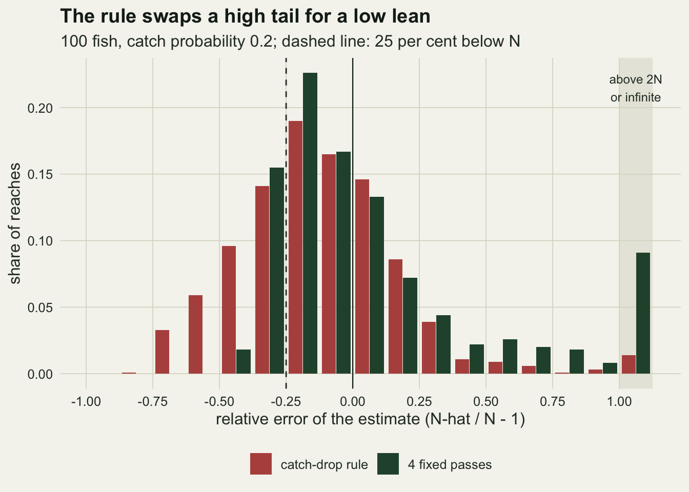
Before the simulation ran, this post fixed the condition under which it would not have been written: a median lean within 0.05 of the matched fixed design and coverage within 3 points of it, both at once, in this cell. The measured gaps are 0.090 and 5.5 points, so the condition is not met.
Why an early stop reads low
The mechanism has a closed-form backbone. The expected catch on pass k is (1 - p) to the power k - 1 times the expected first catch, so the expected sequence first falls to half the first catch at pass 1 + ceiling(log 0.5 / log(1 - p)). A reach whose catches followed their expectations would stop there. Real catches are binomial, and a reach can reach the halfway line earlier by chance: a big first pass, a small second one. Those reaches are exactly the ones whose decline so far is steeper than p implies. The estimate reads a steep decline as a high catch probability, and a high catch probability as few fish left behind, so an early stop is a low estimate. The reaches whose catches happen to fall slowly are fished on, up to the sixth pass, and extra passes are what pull in the high tail that a short fixed design leaves open.
k_expected <- function(p_catch) 1 + ceiling(log(0.5) / log(1 - p_catch))
k_exp_hl   <- k_expected(hl_p)
stop_share <- prop.table(table(factor(rule_r$k, levels = 2:n_pass_max)))
early_share <- mean(rule_r$k < k_exp_hl)
by_stop <- data.frame(
  k      = 2:n_pass_max,
  share  = as.numeric(stop_share),
  med    = as.numeric(tapply(rule_r$rel, factor(rule_r$k, levels = 2:n_pass_max), median)),
  cover  = as.numeric(tapply(rule_r$cover, factor(rule_r$k, levels = 2:n_pass_max), mean)))
stop_cap_share <- by_stop$share[by_stop$k == n_pass_max]
early_med <- median(rule_r$rel[rule_r$k < k_exp_hl])
late_med  <- median(rule_r$rel[rule_r$k >= k_exp_hl])

k2 <- rule_r[rule_r$k == 2, ]
k2_seber   <- k2$c1^2 / (k2$c1 - k2$c2)
k2_ratio_max <- max(k2$nhat / k2$c1)
k2_seber_max <- max(k2_seber / k2$c1)
k2_int_gap   <- max(abs(k2$nhat - k2_seber))
k2_rel_max   <- max(k2$rel)
k2_nhat_frac <- max(k2$nhat) / hl_n
k2_c1_med    <- median(k2$c1) / (hl_n * hl_p)
all_c1_med   <- median(rule_r$c1) / (hl_n * hl_p)
k2_c1_above  <- mean(k2$c1 > hl_n * hl_p)
At a catch probability of 0.2 the expected catches reach half the first at pass 5. Under the rule, 0.589 of reaches stop before that pass, and their median relative error is -0.290; the reaches that stop at pass 5 or later have a median of +0.070. The rule runs to the sixth pass in 0.176 of reaches.
The earliest possible stop can be worked out on paper. When the rule stops at the second pass, the second catch is at most half the first. With two passes the removal estimate is the classical two-pass form c1 squared over (c1 - c2), and with c2 at most c1 / 2 the denominator is at least c1 / 2, so the estimate is at most twice the first catch. The expected first catch is pN, 20 fish here, but a stop at the second pass favours big first catches: among these reaches the median first catch is 1.25 times pN, against 1.00 times pN over all reaches. So the ceiling of twice the first catch sits above 2pN in 0.900 of these reaches, and 2pN is 0.4 of the true number. The chunk checks this against the 90 simulated second-pass stops. The closed-form estimate never exceeds 2.000 times the first catch, the whole-number likelihood maximum sits within 4.1 fish of it and never exceeds 1.875 times the first catch, and the largest relative error among these reaches is -0.40: the biggest second-pass estimate is 0.60 of the true number, still far below it. Their interval covers the truth in 0.367 of cases. That truncation is algebra, not a finding; what the simulation adds is how often it happens and how the rest of the mixture over stopping passes behaves.
stop_df <- rule_r
stop_df$k_fac <- factor(stop_df$k, levels = 2:n_pass_max)
lab_df <- data.frame(k_fac = factor(by_stop$k, levels = 2:n_pass_max),
                     y = 1.25, lab = sprintf("%.0f%%", 100 * by_stop$share))

panel_a <- ggplot(stop_df, aes(k_fac, pmin(rel, 1.2))) +
  geom_hline(yintercept = 0, colour = te_ink, linewidth = 0.4) +
  geom_boxplot(fill = te_gold, colour = te_ink, outlier.size = 0.6,
               linewidth = 0.4, width = 0.6) +
  geom_text(data = lab_df, aes(k_fac, y, label = lab), size = 3.3,
            colour = te_body) +
  scale_y_continuous(limits = c(-0.8, 1.3)) +
  labs(x = "pass at which the rule stopped", y = "relative error",
       title = "A: early stops read low",
       subtitle = "labels: share of reaches") +
  theme_datasheet()

k2_df <- data.frame(c1 = k2$c1, nhat = k2$nhat)
panel_b <- ggplot(k2_df, aes(c1, nhat)) +
  geom_abline(slope = 2, intercept = 0, colour = te_rust, linetype = "dashed",
              linewidth = 0.7) +
  geom_hline(yintercept = hl_n, colour = te_forest, linewidth = 0.6) +
  geom_point(position = position_jitter(width = 0.15, height = 0, seed = 1),
             colour = te_ink, size = 1.4, alpha = 0.7) +
  annotate("text", x = min(k2_df$c1), y = hl_n + 6, label = "true N",
           hjust = 0, colour = te_forest, size = 3.3) +
  annotate("text", x = max(k2_df$c1), y = 2 * max(k2_df$c1) + 4,
           label = "estimate = 2 x first catch", hjust = 1, colour = te_rust,
           size = 3.3) +
  scale_y_continuous(limits = c(0, 110)) +
  labs(x = "first-pass catch", y = "estimate",
       title = "B: second-pass stops",
       subtitle = "dashed: twice the first catch") +
  theme_datasheet()

panel_a + panel_b + plot_layout(widths = c(1.3, 1)) +
  plot_annotation(theme = theme_datasheet())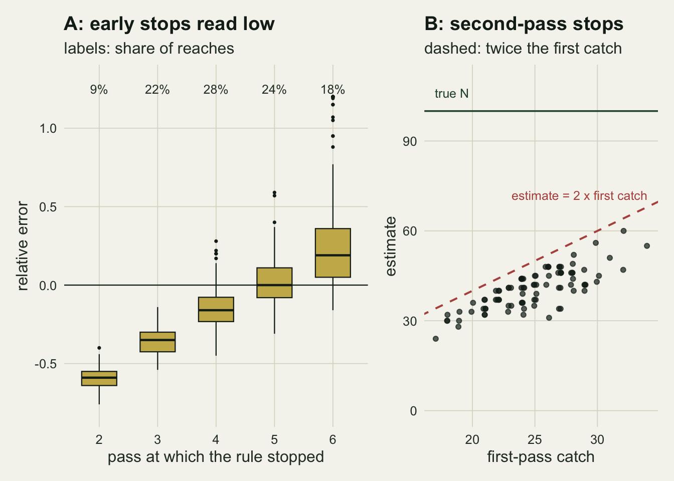
Where it bites
The same comparison runs in all nine cells. The effect depends on how many fish there are to catch and on how fast they come out, and it fades as either of them grows.
cell_cmp <- do.call(rbind, lapply(seq_len(nrow(cells)), function(i) {
  nn <- cells$n_true[i]; pp <- cells$p[i]
  ru <- get_arm(nn, pp, "rule")
  fx <- get_arm(nn, pp, paste0("fixed", match_k(ru$mean_k)))
  k_lo <- floor(ru$mean_k)
  f_lo <- get_arm(nn, pp, paste0("fixed", k_lo))
  f_hi <- get_arm(nn, pp, paste0("fixed", min(k_lo + 1, n_pass_max)))
  data.frame(n_true = nn, p = pp, mean_k = ru$mean_k, k_fix = match_k(ru$mean_k),
             k_exp = k_expected(pp), mae_rule = ru$mae, mae_fix = fx$mae,
             med_rule = ru$med, med_fix = fx$med,
             over_rule = ru$over2, over_fix = fx$over2,
             under_rule = ru$under25, under_fix = fx$under25,
             cov_rule = ru$cover, cov_fix = fx$cover,
             over_lo = f_lo$over2, over_hi = f_hi$over2,
             under_lo = f_lo$under25, under_hi = f_hi$under25,
             cov_lo = f_lo$cover, cov_hi = f_hi$cover)
}))
pick <- function(nn, pp) cell_cmp[cell_cmp$n_true == nn & cell_cmp$p == pp, ]
small_low <- pick(40, 0.2)
big_low   <- pick(300, 0.2)
mid_mid   <- pick(100, 0.3)
mid_high  <- pick(100, 0.5)
small_high <- pick(40, 0.5)
big_high  <- pick(300, 0.5)
high_all  <- cell_cmp[cell_cmp$p == 0.5, ]
high_p    <- high_all[high_all$n_true > 40, ]
under_max_high <- max(c(high_p$under_rule, high_p$under_lo, high_p$under_hi))
cov_gap_high   <- max(abs(c(high_all$cov_rule - high_all$cov_lo,
                            high_all$cov_rule - high_all$cov_hi)))
stop_p5 <- sapply(c(40, 100, 300), function(nn) {
  kk <- get_res(nn, 0.5, "rule")$k
  c(k2 = mean(kk == 2), k3 = mean(kk == 3))
})
At 40 fish and a catch probability of 0.2 the rule fishes 3.71 passes and is set against 4 fixed passes. Its median error is -0.325 against -0.125, and it reports 0.565 of reaches more than a quarter short, against 0.320. The high tail goes from 0.129 to 0.026, and coverage falls from 0.941 to 0.856. Here the typical error grows too: the median absolute relative error is 0.375 under the rule against 0.300. This is the corner where the rule does most harm to the low side: a small population fished inefficiently has noisy early catches, and noise is what triggers early stops.
A bigger population damps the noise in the median and the interval, less so in the low tail. At 300 fish and the same catch probability the rule’s median is -0.050 against -0.027, coverage is 0.942 against 0.956, and the share more than a quarter short is 0.116 against 0.031. At 100 fish and a catch probability of 0.3 the lean is -0.080 against -0.060, but the low tail still more than doubles, 0.192 against 0.085.
A high catch probability removes most of it. At 0.5 the expected catch halves on the second pass, and early stops by chance have little room: the rule stops at the second pass in 0.508 to 0.527 of reaches and at the third in nearly all the rest (0.435 to 0.491). It averages 2.51, 2.50 and 2.49 passes at 40, 100 and 300 fish, halfway between two and three fixed passes, so at this catch probability there is no matched fixed design and the rule is set against both. At 100 and 300 fish no more than 0.011 of reaches come out more than a quarter short under the rule or either fixed design. At 40 fish the rule reports 0.082 of reaches more than a quarter short, against 0.084 for two fixed passes and 0.002 for three. It matches two fixed passes on the low tail and removes their high tail (0.000 against 0.046), and it trails three fixed passes on the low tail. In all three reach sizes the rule’s coverage lies within 1.5 points of both fixed designs, which is the order of the Monte Carlo error. Electrofishing catch probabilities vary widely between species, fish sizes and channels, and the low end, small fish in wide, deep or turbid water, is where this rule needs watching.
tail_df <- rbind(
  data.frame(n_true = cell_cmp$n_true, p = cell_cmp$p, design = "catch-drop rule",
             metric = "above 2N\nor infinite", share = cell_cmp$over_rule),
  data.frame(n_true = cell_cmp$n_true, p = cell_cmp$p, design = "fixed, matched passes",
             metric = "above 2N\nor infinite", share = cell_cmp$over_fix),
  data.frame(n_true = cell_cmp$n_true, p = cell_cmp$p, design = "catch-drop rule",
             metric = "over 25 per cent\nbelow N", share = cell_cmp$under_rule),
  data.frame(n_true = cell_cmp$n_true, p = cell_cmp$p, design = "fixed, matched passes",
             metric = "over 25 per cent\nbelow N", share = cell_cmp$under_fix))
tail_df$p_lab <- factor(sprintf("catch probability %.1f", tail_df$p))
band_df <- rbind(
  data.frame(n_true = cell_cmp$n_true, p = cell_cmp$p, metric = "above 2N\nor infinite",
             lo = pmin(cell_cmp$over_lo, cell_cmp$over_hi),
             hi = pmax(cell_cmp$over_lo, cell_cmp$over_hi)),
  data.frame(n_true = cell_cmp$n_true, p = cell_cmp$p, metric = "over 25 per cent\nbelow N",
             lo = pmin(cell_cmp$under_lo, cell_cmp$under_hi),
             hi = pmax(cell_cmp$under_lo, cell_cmp$under_hi)))
band_df$p_lab <- factor(sprintf("catch probability %.1f", band_df$p))
band_df$band  <- "fixed, neighbouring pass counts"

ggplot(tail_df, aes(n_true, share, colour = design)) +
  geom_ribbon(data = band_df, aes(n_true, ymin = lo, ymax = hi, fill = band),
              inherit.aes = FALSE, alpha = 0.22) +
  geom_line(linewidth = 0.9) +
  geom_point(size = 2.2) +
  facet_grid(metric ~ p_lab) +
  scale_x_log10(breaks = c(40, 100, 300)) +
  scale_colour_manual(values = c(te_rust, te_forest), name = NULL) +
  scale_fill_manual(values = te_forest, name = NULL) +
  labs(x = "fish in the reach (log scale)", y = "share of reaches",
       title = "The rule empties the high tail and fills the low one",
       subtitle = "1000 reaches per point; fixed arm at the rule's rounded mean pass count") +
  theme_datasheet() +
  theme(legend.position = "bottom")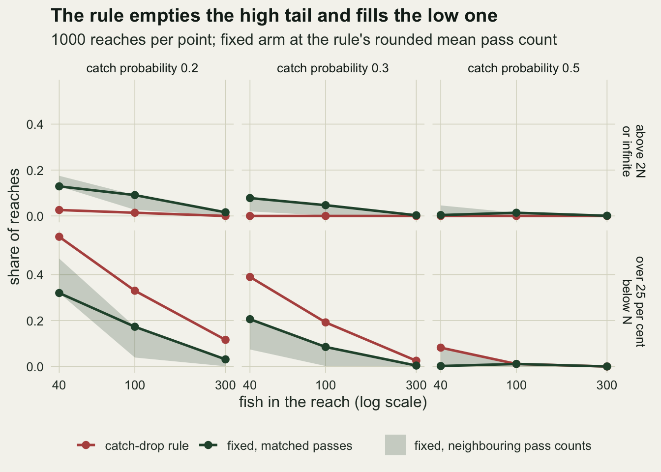
Three repairs, and the fair comparator
Three changes to the rule suggest themselves. One more pass after it triggers gives the estimate a catch that was not used to decide the stop. A minimum of three passes removes the second-pass stops, whose truncation the previous section wrote down. A stricter trigger, a quarter of the first catch instead of half, stops later. Each of them costs passes, so each is compared with fixed passes at its own rounded mean pass count.
repair_arms <- c(rule = "catch-drop rule", rule_plus1 = "rule plus one pass",
                 min3 = "at least three passes", quarter = "quarter trigger")
repair_cmp <- do.call(rbind, lapply(seq_len(nrow(cells)), function(i) {
  nn <- cells$n_true[i]; pp <- cells$p[i]
  do.call(rbind, lapply(names(repair_arms), function(a) {
    ad <- get_arm(nn, pp, a)
    kf <- match_k(ad$mean_k)
    fx <- get_arm(nn, pp, paste0("fixed", kf))
    k_lo <- floor(ad$mean_k)
    f_lo <- get_arm(nn, pp, paste0("fixed", k_lo))
    f_hi <- get_arm(nn, pp, paste0("fixed", min(k_lo + 1, n_pass_max)))
    data.frame(n_true = nn, p = pp, arm = a, label = repair_arms[[a]],
               mean_k = ad$mean_k, k_fix = kf,
               med = ad$med, med_fix = fx$med, cover = ad$cover, cov_fix = fx$cover,
               under = ad$under25, under_fix = fx$under25,
               over = ad$over2, over_fix = fx$over2,
               med_lo = f_lo$med, med_hi = f_hi$med,
               cov_lo = f_lo$cover, cov_hi = f_hi$cover)
  }))
}))
rp <- function(nn, pp, a) repair_cmp[repair_cmp$n_true == nn & repair_cmp$p == pp &
                                       repair_cmp$arm == a, ]
plus_hl  <- rp(hl_n, hl_p, "rule_plus1")
plus_sm  <- rp(40, 0.2, "rule_plus1")
min3_hl  <- rp(hl_n, hl_p, "min3")
min3_sm  <- rp(40, 0.2, "min3")
qrt_hl   <- rp(hl_n, hl_p, "quarter")
qrt_sm   <- rp(40, 0.2, "quarter")
qrt_worst <- repair_cmp[repair_cmp$arm == "quarter", ]
qrt_worst <- qrt_worst[which.max(qrt_worst$cov_fix - qrt_worst$cover), ]

rule_rp  <- rp(hl_n, hl_p, "rule")
excess_rule <- rule_rp$under - rule_rp$under_fix
excess_plus <- plus_hl$under - plus_hl$under_fix

fix6_hl  <- get_arm(hl_n, hl_p, "fixed6")
fix6_r   <- get_res(hl_n, hl_p, "fixed6")
se_cov6  <- paired_se(rule_r$cover, fix6_r$cover)

qrt_r      <- get_res(hl_n, hl_p, "quarter")
qrt_early  <- qrt_r$k < n_pass_max
qrt_early_share <- mean(qrt_early)
qrt_early_cov   <- mean(qrt_r$cover[qrt_early])
fix6_early_cov  <- mean(fix6_r$cover[qrt_early])
One pass beyond the trigger brings the fishing to 5.01 passes at 100 fish and a catch probability of 0.2, and its median error to -0.075, about half the rule’s lean, with coverage of 0.922. The matched design for that effort is 5 fixed passes, which gives -0.040 and 0.945. At 40 fish the same repair fishes 4.56 passes for a median of -0.150 and coverage of 0.906, against -0.100 and 0.931 for 5 fixed passes. The extra pass roughly halves the lean at 100 fish, and it costs as much as a fixed fifth pass that does better on both counts. On the low tail it helps less. At 100 fish it reports 0.164 of reaches more than a quarter short against 0.039 for 5 fixed passes, so the excess over the matched design only falls from 0.157 under the rule to 0.125; at 40 fish the pair is 0.346 against 0.167.
A minimum of three passes fishes 4.34 passes at 100 fish for a median of -0.120 and coverage of 0.929, and at 40 fish 4.12 passes for -0.250 and 0.909. Its matched design is 4 fixed passes in both cells, with a median of -0.050 and coverage of 0.946 at 100 fish and -0.125 and 0.941 at 40. On the low tail the minimum reports 0.290 of reaches more than a quarter short at 100 fish against 0.173, and 0.483 against 0.320 at 40. It removes the worst of the early stops and keeps the rest of the mechanism: every stop from the third pass onwards is still a stop chosen by a steep decline.
The quarter trigger fishes 5.71 passes at 100 fish, close to the six-pass maximum, and its median is -0.040 against -0.030 for 6 fixed passes, with a low tail of 0.072 against 0.008. The lean is almost gone, but the coverage gap is not: 0.918 against 0.940, and at 40 fish 0.865 against 0.931. The largest coverage shortfall of the quarter trigger in the grid is 6.6 points, at 40 fish and a catch probability of 0.2. A stricter trigger still stops on a catch that happens to be small, and the interval, built as if the number of passes had been fixed, is too short for those reaches. At 100 fish the quarter trigger stops before the sixth pass in 0.200 of reaches; on those reaches its interval covers the truth in 0.715 of cases, against 0.825 for six fixed passes on the same catches, and on every other reach it is six fixed passes.
The statistician’s question is whether fixed passes at the rule’s mean effort are the fair comparison, or fixed passes at its maximum. Six fixed passes is what a crew prepared to go to six could always have done. At 100 fish and a catch probability of 0.2, six fixed passes give a median of -0.030, coverage of 0.940 (4.9 points above the rule, paired standard error 1.1 points), and 0.008 of reaches more than a quarter short. That comparison is lopsided by construction, since the rule’s point is to save passes. Matched mean effort answers the question a field crew is asking, which is what the same afternoon of fishing buys when it is spent by rule instead of by plan.
rep_long <- rbind(
  data.frame(repair_cmp[, c("n_true", "p", "label")],
             metric = "median\nerror gap",
             gap = repair_cmp$med - repair_cmp$med_fix,
             g_lo = repair_cmp$med - pmax(repair_cmp$med_lo, repair_cmp$med_hi),
             g_hi = repair_cmp$med - pmin(repair_cmp$med_lo, repair_cmp$med_hi)),
  data.frame(repair_cmp[, c("n_true", "p", "label")],
             metric = "coverage\ngap",
             gap = repair_cmp$cover - repair_cmp$cov_fix,
             g_lo = repair_cmp$cover - pmax(repair_cmp$cov_lo, repair_cmp$cov_hi),
             g_hi = repair_cmp$cover - pmin(repair_cmp$cov_lo, repair_cmp$cov_hi)))
rep_long$label  <- factor(rep_long$label, levels = unname(repair_arms))
rep_long$metric <- factor(rep_long$metric, levels = c("median\nerror gap", "coverage\ngap"))
rep_long$p_lab  <- factor(sprintf("catch probability %.1f", rep_long$p))

dodge_x <- position_dodge(width = 0.12)
ggplot(rep_long, aes(n_true, gap, colour = label, linetype = label, shape = label)) +
  geom_hline(yintercept = 0, colour = te_ink, linewidth = 0.4) +
  geom_linerange(aes(ymin = g_lo, ymax = g_hi), linewidth = 0.5, alpha = 0.6,
                 linetype = "solid", position = dodge_x) +
  geom_line(linewidth = 0.8, position = dodge_x) +
  geom_point(size = 2, position = dodge_x) +
  facet_grid(metric ~ p_lab, scales = "free_y") +
  scale_x_log10(breaks = c(40, 100, 300)) +
  scale_colour_manual(values = c(te_rust, te_gold, te_forest, te_ink), name = NULL) +
  scale_linetype_manual(values = c("solid", "solid", "solid", "22"), name = NULL) +
  scale_shape_manual(values = c(16, 17, 15, 1), name = NULL) +
  labs(x = "fish in the reach (log scale)", y = "difference from matched fixed passes",
       title = "Repairs cut the lean, not all of the coverage gap",
       subtitle = "1000 reaches per point, same catches for every design") +
  theme_datasheet() +
  theme(legend.position = "bottom") +
  guides(colour = guide_legend(nrow = 2))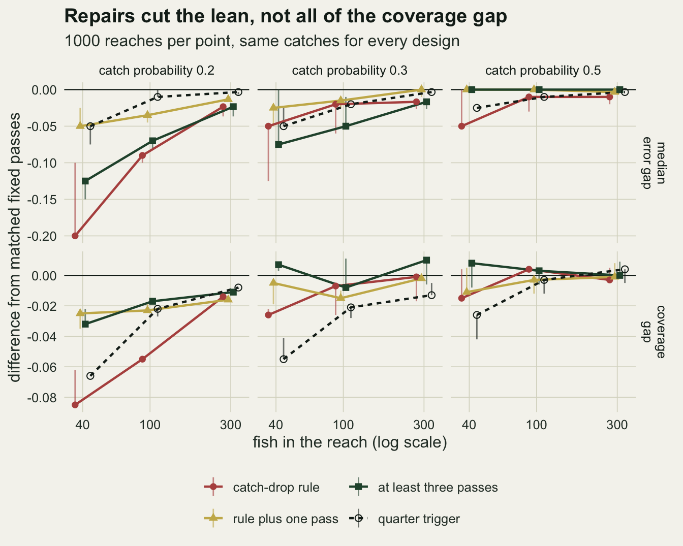
What to report
Report how the number of passes was decided, in words a reader can apply: fixed in advance, or run until a catch was at most some fraction of the first, with the minimum and the maximum. Without that sentence a reader cannot tell whether a reach with a two-pass estimate had a short plan or a steep early decline, and the second kind of two-pass estimate is bounded by twice the first catch whatever the population.
When the passes are decided by the catches, the profile interval is not the interval it looks like. At a catch probability of 0.2 it covered the true number in 0.891 of reaches of 100 fish, not 0.95, and at 40 fish in 0.856. If an estimate is going to be set against a management threshold, say so, and treat a result a quarter or more below the threshold with the knowledge that the rule reports that outcome in 0.330 of reaches that actually sit at 100 fish, against 0.173 for the same effort fished to a plan.
The cheapest remedy is to decide the number of passes before the first one and keep to it. Where the protocol must stay adaptive, fish at least one pass beyond the trigger. At 100 fish that halves the median lean, but it still reports about 4 times as many reaches a quarter short as the same effort fished to a plan. State also the catch probability the data imply, since the damage is concentrated where that probability is low.
Honest limits
Every reach here is closed and every fish has the same catch probability on every pass. Real electrofishing breaks both, most often with a catchability that falls over passes, which pushes the estimate low on its own; Removal estimates when catchability falls measures that. The two sources of lean were not run together, and there is no reason to expect them to add simply, because a falling catchability also changes when the catch halves.
rmse_fin <- function(rel) sqrt(mean(rel[is.finite(rel)]^2))
rmse_rule <- rmse_fin(rule_r$rel)
rmse_fix  <- rmse_fin(fix_r$rel)
mc_se_cov <- sqrt(0.9 * 0.1 / n_reach)
The estimator is the whole-number Zippin maximum with a search that stops at 20T + 100 fish, and a maximum at that ceiling is scored as infinite. The high-tail share counts those, so it does not depend on where the ceiling sits as long as it is far above 2N. A root mean squared error would: over the finite estimates at this ceiling it is 0.574 for the rule and 0.960 for 4 fixed passes at 100 fish and a catch probability of 0.2, and a higher ceiling lets larger finite estimates into the fixed design’s figure. For that reason the post reports tail shares and medians, not a mean squared error. The Carle and Strub estimator, which tames the infinite estimates of flat catch sequences with a prior on the catch probability, was not run.
The rule is one rule. Field versions differ in the fraction, in whether the comparison is with the first pass or the previous one, in the minimum and maximum, and in whether a crew also stops because a catch was zero. No published agency protocol that writes a fixed fraction of the first catch as the stopping criterion was found for this post, so the rule is framed here as this site’s own advice and a common field habit, and the half and quarter triggers are illustrations. Only a trigger at a half or a quarter of the first catch was simulated, with six passes as the maximum.
The grid has three population sizes and three catch probabilities, 1000 reaches each. The Monte Carlo standard error of a coverage of 0.9 on 1000 reaches is 0.9 points, and the headline comparisons carry paired standard errors computed from the same catches. Coverage differences in the high-probability cells are of that order and are not interpreted.
References
Zippin C 1958 Journal of Wildlife Management 22(1):82-90 (10.2307/3797301)
Whitehead J 1986 Biometrika 73(3):573-581 (10.1093/biomet/73.3.573)
Rubin DB 1976 Biometrika 63(3):581-592 (10.1093/biomet/63.3.581)
Riley SC, Fausch KD 1992 North American Journal of Fisheries Management 12(4):768-776 (10.1577/1548-8675(1992)012<0768:UOTPSB>2.3.CO;2)