library(ggplot2)
library(patchwork)

te_paper  <- "#f5f4ee"
te_ink    <- "#16241d"
te_body   <- "#2c3a31"
te_forest <- "#275139"
te_rust   <- "#b5534e"
te_gold   <- "#c9b458"
te_line   <- "#dad9ca"

theme_datasheet <- function() {
  theme_minimal(base_size = 12) +
    theme(plot.background  = element_rect(fill = te_paper, colour = NA),
          panel.background = element_rect(fill = te_paper, colour = NA),
          panel.grid.major = element_line(colour = te_line, linewidth = 0.3),
          panel.grid.minor = element_blank(),
          text             = element_text(colour = te_body),
          plot.title       = element_text(colour = te_ink, face = "bold"),
          plot.subtitle    = element_text(colour = te_body),
          axis.text        = element_text(colour = te_body),
          strip.text       = element_text(colour = te_ink, face = "bold"))
}Missing values in a predictor: why, not how many
R
missing data
multiple imputation
regression
simulation
ecology tutorial
With 40 per cent of a predictor blank, the reason for the gap decides whether deletion or multiple imputation is right. A simulation in R for field ecologists.
A grassland survey has five hundred plots, a biomass harvest from every one, and a soil moisture reading that is meant to explain it. At the end of the season the moisture column is forty per cent blank. There are two quite different ways that can happen. In one survey the handheld probe will not go into dry, hard ground, so the driest plots have no reading. In the other the moisture was measured from cores sent to a laboratory, and the field team only cored the plots whose sward looked rich. The spreadsheet looks the same in both: the same number of blanks, in the same column, and the same response fully recorded.
This site has already put gaps into a predictor twice. AIC with missing values: the silent row drop blanks two predictors completely at random to study how many rows each candidate model keeps. Multiple imputation by chained equations blanks both the predictor and the response, drives the gaps with an auxiliary variable that sits in the imputation model and not in the analysis model, and finds across four hundred replicates that complete-case analysis, single imputation and multiple imputation are all unbiased for the slope, differing only in their intervals. That result is correct, and it is a case where the question of this post does not arise. This post asks what happens when the reason is the predictor itself, or the response.
The three posts closest to this one put the hole in the response. Missing data: MCAR, MAR and MNAR blanks the response under each of Rubin’s three mechanisms and finds complete-case deletion safe for the slope under missing at random and broken under missing not at random. Single imputation: bias and variance and Checking missing-data assumptions both let the chance of a missing response depend on the predictor. With the hole in the predictor the verdict of the first of those turns over, and the logistic missingness check from the last of them turns out to be unable to say which way round the world is. The AIC post is about a different question, the row counts that differ between candidate models, and its passing remark that complete cases are unbiased only when values are missing completely at random is stricter than it needs to be for a regression slope, as the next section shows.
None of this is new. Little 1992 reviewed regression with missing predictors and stated the condition under which complete-case analysis is consistent; White and Carlin 2010 ran the head-to-head of multiple imputation against complete-case analysis for missing covariates and found that each can win depending on the mechanism. This post is a demonstration of their result on an ecological design, with the imputation coded by hand, not a claim to it. What is measured here is how large the damage is at a realistic share of blanks, whether the obvious rescues rescue anything, and whether the observed data can tell the reader which of the two surveys they are holding.
The theory says which rows are safe to drop
A regression of biomass on moisture estimates the mean of biomass given moisture. Deleting rows changes which moisture values are in the sample, and that is harmless as long as, among plots with the same moisture, the kept rows and the deleted rows have the same biomass on average. Little 1992 states it as the condition that complete-case regression is consistent when the probability that the predictor is missing does not depend on the response once the predictor is known. It may depend on the predictor itself as strongly as it likes.
That is the whole theory, and it already says which survey is which. The probe fails because the moisture is low, so the missingness depends on the predictor only, and deletion is safe. The laboratory cores were chosen by looking at the biomass, so the missingness depends on the response, and deletion is not. In Rubin’s 1976 vocabulary the probe survey is missing not at random, since the blank depends on the value that is blank, and the laboratory survey is missing at random, since it depends only on something recorded. Multiple imputation is built for missing at random, and the labels therefore point to the opposite verdict from the one the theory gives for deletion. The simulation below measures both halves.
Five hundred plots and three reasons for a blank
Moisture is standardised to mean zero and unit standard deviation, and biomass rises by two units per standard deviation of moisture with residual noise of standard deviation two. Those constants and everything else in the next chunk were fixed before any result was looked at.
n_plot  <- 500     # plots per season
b0      <- 5       # biomass at average moisture
b1      <- 2       # the slope the analysis is after
sig_e   <- 2       # residual standard deviation of biomass
m_imp   <- 20      # imputations per data set
n_draw  <- 200     # fresh data sets per cell of the grid
share_main <- 0.4  # share of rows with moisture blank, main case
shares  <- c(0.2, 0.4, 0.6)
k_soft  <- 2       # slope of the soft probe failure curve, per sd of moisture
rho_w   <- 0.7     # correlation of the auxiliary wetness index with moisture

calib <- function(lin, share) {
  a <- uniroot(function(a) mean(plogis(a + lin)) - share, c(-30, 30))$root
  plogis(a + lin)
}

make_season <- function(case, share) {
  x <- rnorm(n_plot)
  y <- b0 + b1 * x + rnorm(n_plot, 0, sig_e)
  w <- rho_w * x + sqrt(1 - rho_w^2) * rnorm(n_plot)
  mx <- switch(case,
    probe = , probe_aux = x < quantile(x, share),        # no reading below a floor
    probe_soft = runif(n_plot) < calib(-k_soft * x, share),
    lab   = runif(n_plot) < calib(-(y - mean(y)), share), # cored where the sward looked rich
    lost  = runif(n_plot) < share)                       # a box of cores lost
  list(x = x, y = y, w = w, mx = mx, case = case)
}
The probe case blanks every plot below the chosen percentile of its own moisture, which is the sharpest possible form of a value causing its own absence. The soft probe case replaces the hard floor by a logistic failure curve in moisture, calibrated to the same share. The laboratory case blanks a plot with a probability that falls with its biomass, again calibrated to the same share. The lost case is the control: a box of cores dropped in a river, blank completely at random. A fifth case keeps the hard probe floor and adds a wetness index from a terrain model, known for every plot, correlated with moisture and playing no direct part in which plots were blank.
Three estimators are applied to every data set. Complete-case analysis is ordinary least squares on the rows with a moisture reading. Multiple imputation draws the missing moisture values from a regression of moisture on biomass (and on the wetness index where it exists) fitted to the observed rows, drawing the regression coefficients and residual variance from their posterior first, so that each imputation is proper; the slope is then fitted to each of the 20 completed data sets and pooled by Rubin’s rules with the Barnard and Rubin degrees of freedom. This is the same machinery the chained-equations post builds, reduced to one incomplete variable. The third estimator, used in one row of one table only, is the deterministic regression fill from the single-imputation post.
slr <- function(xv, yv) {
  dx <- xv - mean(xv); sxx <- sum(dx^2)
  bh <- sum(dx * (yv - mean(yv))) / sxx
  rss <- sum((yv - mean(yv) - bh * dx)^2)
  c(b = bh, se = sqrt(rss / (length(xv) - 2) / sxx), dfr = length(xv) - 2)
}

imp_draw <- function(target, miss, preds) {
  o <- !miss; xo <- cbind(1, preds[o, , drop = FALSE]); v <- target[o]
  xtxi <- chol2inv(chol(crossprod(xo))); bh <- xtxi %*% crossprod(xo, v)
  dfr <- sum(o) - ncol(xo); s2 <- sum((v - xo %*% bh)^2) / dfr
  s2_star <- s2 * dfr / rchisq(1, dfr)
  b_star <- bh + t(chol(s2_star * xtxi)) %*% rnorm(ncol(xo))
  out <- target
  out[miss] <- as.numeric(cbind(1, preds[miss, , drop = FALSE]) %*% b_star) +
    rnorm(sum(miss), 0, sqrt(s2_star))
  out
}

rubin <- function(q, u, m, nu_com) {
  qbar <- mean(q); ubar <- mean(u^2); bvar <- var(q)
  tvar <- ubar + (1 + 1 / m) * bvar
  lam <- (1 + 1 / m) * bvar / tvar
  nu_old <- (m - 1) / lam^2
  nu_obs <- (nu_com + 1) / (nu_com + 3) * nu_com * (1 - lam)
  c(q = qbar, se = sqrt(tvar), dfr = nu_old * nu_obs / (nu_old + nu_obs))
}

analyse <- function(s) {
  o <- !s$mx
  cc <- slr(s$x[o], s$y[o]); t_cc <- qt(0.975, cc["dfr"])
  preds <- if (s$case == "probe_aux") cbind(s$y, s$w) else cbind(s$y)
  q <- u <- numeric(m_imp)
  for (k in seq_len(m_imp)) {
    f <- slr(imp_draw(s$x, s$mx, preds), s$y); q[k] <- f["b"]; u[k] <- f["se"]
  }
  p <- rubin(q, u, m_imp, n_plot - 2); t_mi <- qt(0.975, p["dfr"])
  fill <- lm.fit(cbind(1, preds[o, , drop = FALSE]), s$x[o])$coefficients
  x_fill <- s$x
  x_fill[s$mx] <- as.numeric(cbind(1, preds[s$mx, , drop = FALSE]) %*% fill)
  si <- slr(x_fill, s$y); t_si <- qt(0.975, si["dfr"])
  g_diag <- summary(glm(s$mx ~ s$y, family = binomial))$coefficients
  unname(c(mean(s$mx),
           cc["b"], cc["b"] - t_cc * cc["se"], cc["b"] + t_cc * cc["se"],
           p["q"], p["q"] - t_mi * p["se"], p["q"] + t_mi * p["se"],
           si["b"], si["b"] - t_si * si["se"], si["b"] + t_si * si["se"],
           g_diag[2, 4], g_diag[2, 1]))
}
out_names <- c("blank_share", "cc", "cc_lo", "cc_hi", "mi", "mi_lo", "mi_hi",
               "si", "si_lo", "si_hi", "p_diag", "b_diag")
One season of each
Before the repeated simulation, one season from each of the two surveys that matter, with the same share of plots blank.
set.seed(4417)
one_probe <- make_season("probe", share_main)
one_lab   <- make_season("lab", share_main)
fit_probe <- setNames(analyse(one_probe), out_names)
fit_lab   <- setNames(analyse(one_lab), out_names)
imp_x_fit <- function(s) coef(lm(s$x[!s$mx] ~ s$y[!s$mx]))
full_x_fit <- function(s) coef(lm(s$x ~ s$y))
ix_probe <- imp_x_fit(one_probe); fx_probe <- full_x_fit(one_probe)
ix_lab   <- imp_x_fit(one_lab);   fx_lab   <- full_x_fit(one_lab)
round(rbind(probe = fit_probe[c("blank_share", "cc", "mi")],
            lab   = fit_lab[c("blank_share", "cc", "mi")]), 3)
blank_share cc mi
probe 0.400 1.843 2.395
lab 0.418 1.496 1.977In the probe season 40 per cent of plots have no moisture reading. Complete-case regression on the rest returns a slope of 1.843 against the generating 2, and multiple imputation returns 2.395, so deletion is the nearer of the two, by 0.157 against 0.395. In the laboratory season, with 42 per cent blank, the order reverses: complete-case gives 1.496 and multiple imputation 1.977, off by 0.504 and 0.023. One season could be luck, which is what the next section is for.
The reason is visible in the regression the imputation model is built on. Imputing moisture needs a regression of moisture on biomass, fitted to the plots that have a reading. In the full probe season, blanks included, that regression has a slope of 0.256 moisture units per unit of biomass; fitted to the plots the probe could read it has 0.147. Truncating moisture from below flattens every regression that has moisture on the left-hand side, so the imputation model draws the dry plots’ moisture too close to the observed range, the completed moisture values are squeezed together, and a slope fitted to squeezed values comes out too steep. In the laboratory season the same regression is fitted to plots selected on biomass, which is its own right-hand side, and conditioning on the right-hand side is exactly what a regression tolerates: 0.255 on the observed plots against 0.242 in the full season. Each estimator is safe when the selection falls on its own predictor.
season_frame <- function(s, label) {
  data.frame(x = s$x, y = s$y,
             status = ifelse(s$mx, "blank (true value)", "recorded"),
             survey = label)
}
lab_probe <- "Probe fails in dry soil"
lab_lab   <- "Cores taken where sward looked rich"
pts <- rbind(season_frame(one_probe, lab_probe), season_frame(one_lab, lab_lab))
pts$survey <- factor(pts$survey, levels = c(lab_probe, lab_lab))
lines_df <- data.frame(
  survey = factor(rep(c(lab_probe, lab_lab), each = 2), levels = c(lab_probe, lab_lab)),
  fit = rep(c("complete case", "multiple imputation"), 2),
  slope = c(fit_probe["cc"], fit_probe["mi"], fit_lab["cc"], fit_lab["mi"]))
anchor <- function(s) {
  x_comp <- mean(replicate(m_imp, mean(imp_draw(s$x, s$mx, cbind(s$y)))))
  c(mean(s$x[!s$mx]), mean(s$y[!s$mx]), x_comp, mean(s$y))
}
set.seed(4418)
anc <- rbind(anchor(one_probe), anchor(one_lab))
lines_df$intercept <- c(anc[1, 2] - fit_probe["cc"] * anc[1, 1],
                        anc[1, 4] - fit_probe["mi"] * anc[1, 3],
                        anc[2, 2] - fit_lab["cc"] * anc[2, 1],
                        anc[2, 4] - fit_lab["mi"] * anc[2, 3])
ggplot(pts, aes(x, y)) +
  geom_point(aes(shape = status, colour = status), size = 1.3, alpha = 0.8) +
  geom_abline(intercept = b0, slope = b1, colour = te_ink, linetype = "dashed",
              linewidth = 0.7) +
  geom_abline(data = lines_df, aes(intercept = intercept, slope = slope, colour = fit),
              linewidth = 1.1) +
  facet_wrap(~ survey) +
  scale_shape_manual(values = c("blank (true value)" = 1, "recorded" = 16), name = NULL) +
  scale_colour_manual(values = c("blank (true value)" = "#9a9a8c", "recorded" = te_body,
                                 "complete case" = te_forest,
                                 "multiple imputation" = te_rust), name = NULL) +
  guides(shape = "none",
         colour = guide_legend(override.aes = list(shape = c(1, NA, NA, 16),
                                                   linetype = c(0, 1, 1, 0)))) +
  labs(x = "soil moisture (standardised)", y = "biomass",
       title = "Same share blank, opposite winners",
       subtitle = "dashed: the generating line") +
  theme_datasheet() + theme(legend.position = "bottom")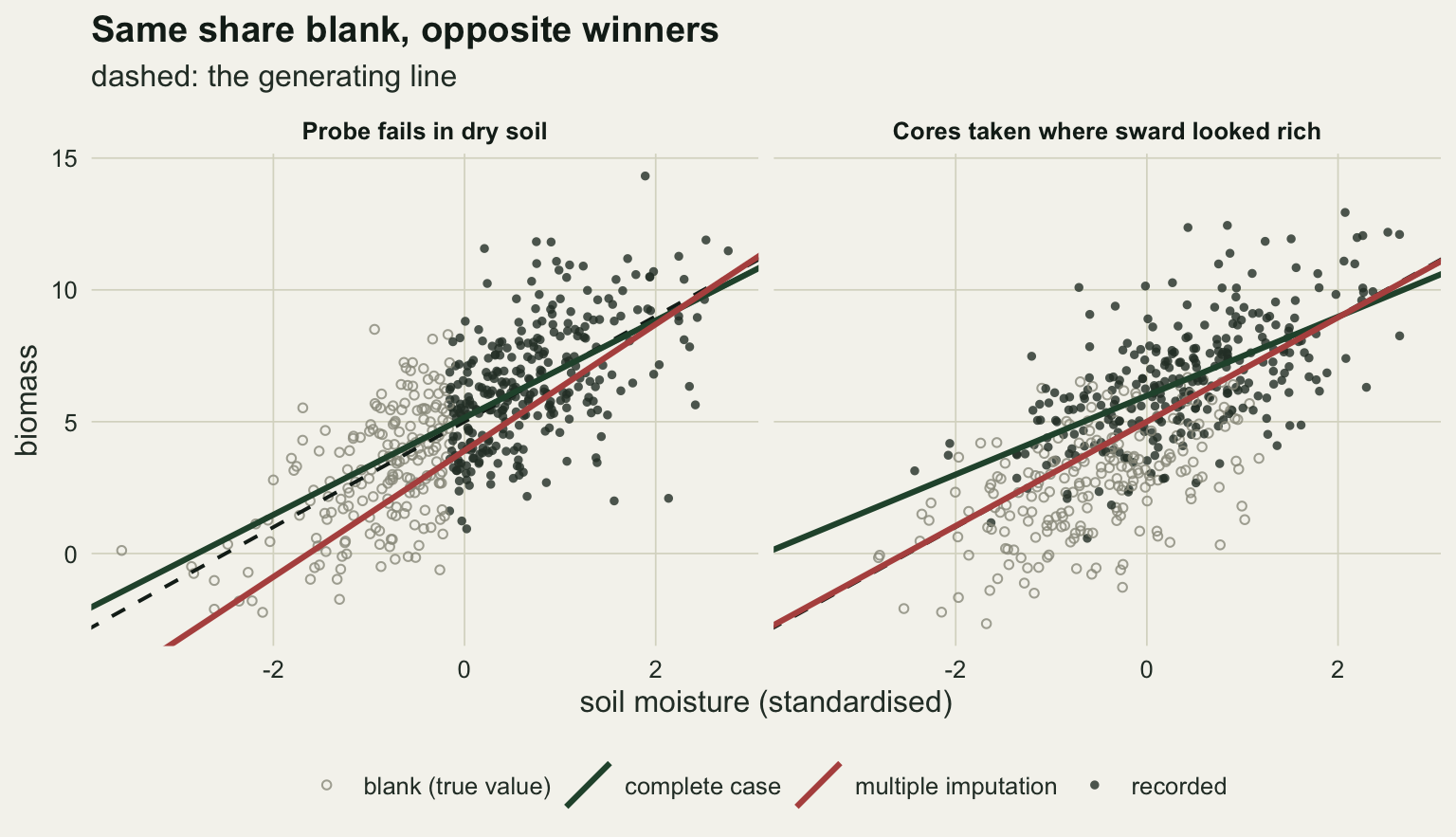
Two hundred seasons
One season is one draw. The same pair of surveys and the lost-box control, each repeated on 200 fresh data sets, with the soft probe, the auxiliary and the other two shares run in the same loop for the sections that follow.
cells <- expand.grid(case = c("probe", "probe_soft", "lab", "lost", "probe_aux"),
                     share = shares, stringsAsFactors = FALSE)
set.seed(20260926)
sims <- lapply(seq_len(nrow(cells)), function(i) {
  r <- t(replicate(n_draw, analyse(make_season(cells$case[i], cells$share[i]))))
  colnames(r) <- out_names
  data.frame(case = cells$case[i], share = cells$share[i], draw = seq_len(n_draw), r)
})
all_draws <- do.call(rbind, sims)

summ <- function(d) {
  data.frame(case = d$case[1], share = d$share[1], rows_blank = mean(d$blank_share),
    cc_med = median(d$cc), cc_lo = min(d$cc), cc_hi = max(d$cc),
    cc_bias = median(d$cc) - b1, cc_cover = mean(d$cc_lo <= b1 & b1 <= d$cc_hi),
    cc_width = mean(d$cc_hi - d$cc_lo),
    mi_med = median(d$mi), mi_lo = min(d$mi), mi_hi = max(d$mi),
    mi_bias = median(d$mi) - b1, mi_cover = mean(d$mi_lo <= b1 & b1 <= d$mi_hi),
    mi_width = mean(d$mi_hi - d$mi_lo),
    si_bias = median(d$si) - b1, si_cover = mean(d$si_lo <= b1 & b1 <= d$si_hi),
    diag_rate = mean(d$p_diag < 0.05), diag_neg = mean(d$b_diag < 0), gap_pos = mean(d$mi > d$cc),
    gap_med = median(d$mi - d$cc))
}
tab <- do.call(rbind, lapply(sims, summ))
row_of <- function(cs, sh = share_main) tab[tab$case == cs & abs(tab$share - sh) < 1e-9, ]
tp <- row_of("probe"); tl <- row_of("lab"); tc <- row_of("lost")
mcse_95 <- sqrt(0.95 * 0.05 / n_draw)
over_pct <- 100 * tp$mi_bias / b1
main_tab <- rbind(tp, tl, tc)[, c("case", "cc_bias", "cc_cover", "cc_width",
                                  "mi_bias", "mi_cover", "mi_width", "si_bias", "si_cover")]
main_tab[, -1] <- round(main_tab[, -1], 3)
main_tab
case cc_bias cc_cover cc_width mi_bias mi_cover mi_width si_bias si_cover
6 probe 0.015 0.945 0.695 0.498 0.190 0.686 1.335 0.000
8 lab -0.536 0.005 0.439 -0.010 0.960 0.416 0.490 0.005
9 lost -0.010 0.930 0.457 -0.014 0.935 0.414 0.497 0.000The denominators first, because they are the easiest pair in the missing-data literature to confuse. Coverage below is the share of the 200 fresh data sets per cell whose 95 per cent interval contains the generating slope, never a share of the 20 imputations inside one data set. Bias is the median slope across those data sets minus 2.00. The share blank is the share of plots, that is of rows, with no moisture reading; here the realised share averages 0.400 in the probe survey and 0.400 in the laboratory survey. With 200 data sets the Monte Carlo standard error of a coverage near its nominal value is 0.015.
In the probe survey complete-case analysis has a median slope of 2.015, a bias of +0.015, estimates ranging from 1.425 to 2.407 across data sets, and coverage of 0.945. Multiple imputation has a median of 2.498, 25 per cent above the truth, a range from 1.972 to 2.848, and coverage of 0.190. The percentage is scale free only because the target is a slope; the same bias on an intercept would have to be read against its own units.
In the laboratory survey the two swap. Complete-case analysis has a median of 1.464, a bias of -0.536 and coverage of 0.005; multiple imputation a median of 1.990, a bias of -0.010 and coverage of 0.960. The lost-box control is the case the swap is read against: both are unbiased (-0.010 and -0.014) and both cover (0.930 and 0.935), with the imputation interval narrower on average, 0.414 against 0.457, because it uses the biomass of the plots that lost their reading. That is the chained-equations post’s result, and it is what both methods look like when the reason for the blank does not matter.
The deterministic fill does badly in all three. It puts every missing moisture value exactly on the regression of moisture on biomass, with none of the scatter real moisture has around that line, and its slope is +0.490 off even in the laboratory survey where a proper imputation from the same regression is unbiased, with coverage of 0.005. Under the random losses its bias is +0.497, and in the probe survey +1.335. The single-imputation post shows the milder form with the hole in the response: the fill lies on the line, so the slope survives, but the correlation is inflated and the reported standard error shrinks. Here the filled variable is the one the slope is divided by, so the squeeze moves the slope itself.
n_show <- 60
iv <- all_draws[all_draws$case %in% c("probe", "lab") &
                abs(all_draws$share - share_main) < 1e-9 & all_draws$draw <= n_show, ]
iv_long <- rbind(
  data.frame(case = iv$case, draw = iv$draw, est = iv$cc, lo = iv$cc_lo, hi = iv$cc_hi,
             estimator = "complete case"),
  data.frame(case = iv$case, draw = iv$draw, est = iv$mi, lo = iv$mi_lo, hi = iv$mi_hi,
             estimator = "multiple imputation"))
iv_long$covers <- ifelse(iv_long$lo <= b1 & b1 <= iv_long$hi, "covers", "misses")
iv_long$case <- factor(ifelse(iv_long$case == "probe", lab_probe, lab_lab),
                       levels = c(lab_probe, lab_lab))
ggplot(iv_long, aes(draw, est, colour = covers)) +
  geom_hline(yintercept = b1, colour = te_ink, linewidth = 0.6) +
  geom_errorbar(aes(ymin = lo, ymax = hi), width = 0, linewidth = 0.5) +
  geom_point(size = 0.9) +
  facet_grid(estimator ~ case) +
  scale_colour_manual(values = c(covers = te_forest, misses = te_rust), name = NULL) +
  labs(x = "data set", y = "estimated slope",
       title = "The reason for the blank picks the estimator",
       subtitle = "horizontal line: the generating slope") +
  theme_datasheet() + theme(legend.position = "bottom")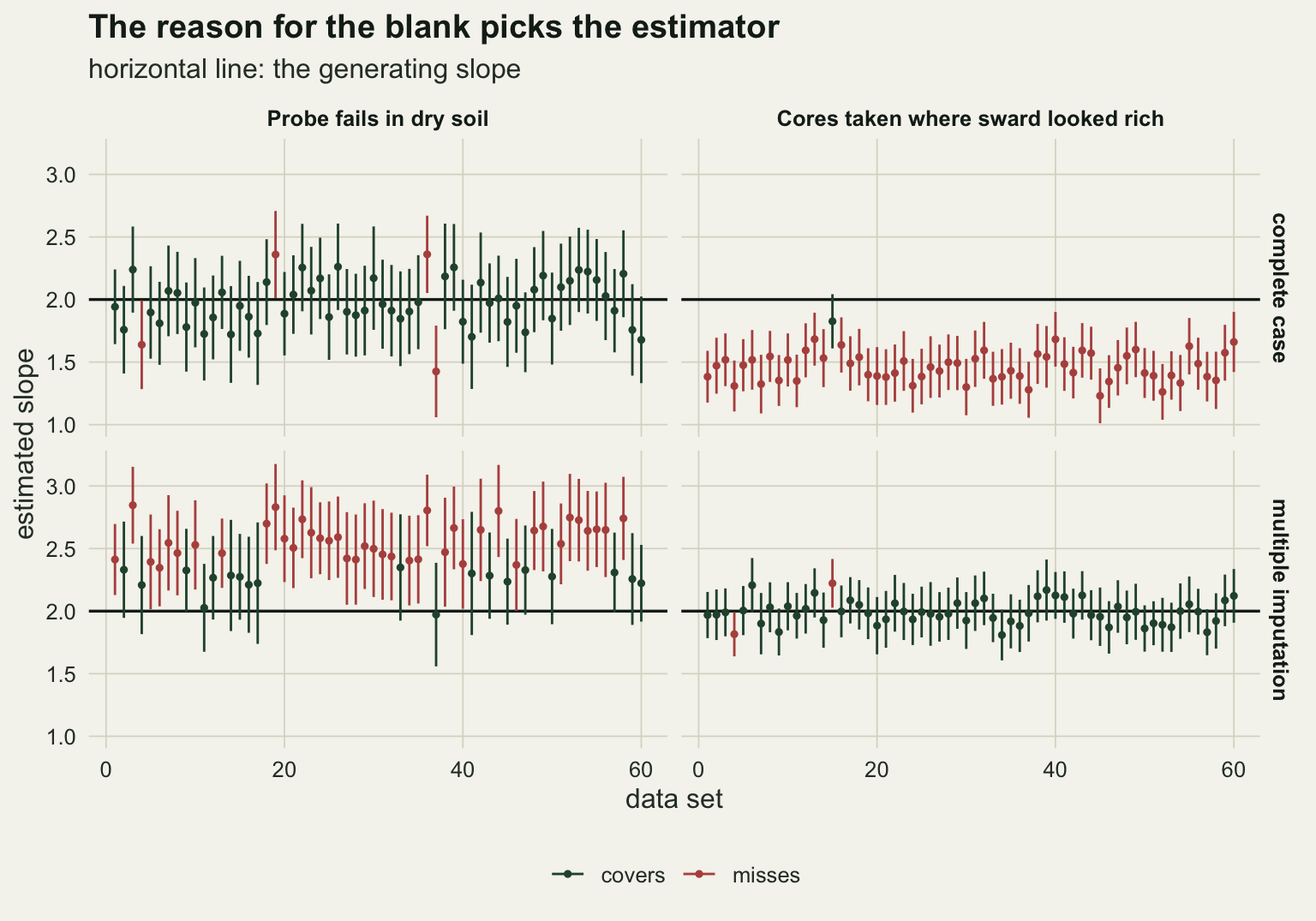
The amount sets the size of the damage, not the winner
The obvious objection is that forty per cent is a lot, and that at a smaller share the difference between the estimators would stop mattering. The grid runs every case at three shares.
grid_tab <- tab[, c("case", "share", "cc_bias", "cc_cover", "mi_bias", "mi_cover")]
grid_tab[, -(1:2)] <- round(grid_tab[, -(1:2)], 3)
grid_tab[order(grid_tab$case, grid_tab$share), ]
case share cc_bias cc_cover mi_bias mi_cover
3 lab 0.2 -0.349 0.065 0.001 0.945
8 lab 0.4 -0.536 0.005 -0.010 0.960
13 lab 0.6 -0.656 0.000 -0.025 0.955
4 lost 0.2 -0.015 0.935 -0.013 0.955
9 lost 0.4 -0.010 0.930 -0.014 0.935
14 lost 0.6 0.008 0.985 0.006 0.960
1 probe 0.2 0.004 0.970 0.292 0.375
6 probe 0.4 0.015 0.945 0.498 0.190
11 probe 0.6 0.019 0.925 0.672 0.275
5 probe_aux 0.2 0.003 0.960 0.295 0.305
10 probe_aux 0.4 -0.002 0.960 0.527 0.055
15 probe_aux 0.6 0.031 0.945 0.761 0.040
2 probe_soft 0.2 -0.006 0.945 0.137 0.745
7 probe_soft 0.4 -0.015 0.935 0.215 0.635
12 probe_soft 0.6 -0.003 0.975 0.273 0.610tp_lo <- row_of("probe", 0.2); tp_hi <- row_of("probe", 0.6)
tl_lo <- row_of("lab", 0.2); tl_hi <- row_of("lab", 0.6)
ts <- row_of("probe_soft"); ts_lo <- row_of("probe_soft", 0.2); ts_hi <- row_of("probe_soft", 0.6)
ta <- row_of("probe_aux"); ta_lo <- row_of("probe_aux", 0.2); ta_hi <- row_of("probe_aux", 0.6)
cc_probe_worst <- max(abs(tab$cc_bias[tab$case %in% c("probe", "probe_soft", "probe_aux")]))
cc_probe_cov_min <- min(tab$cc_cover[tab$case %in% c("probe", "probe_soft", "probe_aux")])In the probe survey the multiple imputation bias grows with the share blank, from +0.292 at 20 per cent to +0.672 at 60 per cent, with coverage between 0.190 and 0.375. In the laboratory survey the complete-case bias grows the same way, from -0.349 to -0.656, with coverage no higher than 0.065. So the amount sets how badly the wrong method does. It never changes which method is wrong: at every share the probe survey is won by deletion and the laboratory survey by imputation.
A probe does not fail at a knife edge. With the hard floor replaced by a logistic failure curve (a slope of 2 on the logit scale per standard deviation of moisture), complete-case analysis is untouched, as the theory says it must be, since the blank still depends on moisture alone: its largest absolute bias across all the probe variants and shares is 0.031 and its lowest coverage 0.925. What moves is the imputation. At forty per cent the soft probe’s multiple imputation bias is +0.215 with coverage of 0.635, against +0.498 and 0.190 for the hard floor. A softer failure curve blurs the truncation the imputation model inherits, so the damage shrinks, but it does not vanish at any share in the grid: from +0.137 to +0.273.
An auxiliary does not rescue the imputation
The imputation model so far has only biomass to impute moisture from, which is the worst model an ecologist would build. The standard advice from the imputation literature is to add auxiliary variables, and the wetness index is exactly that: known for every plot, correlated with moisture at 0.7, and with no direct role in which plots the probe could read.
With the wetness index in the imputation model and the hard probe floor, multiple imputation has a bias of +0.527 and coverage of 0.055 at forty per cent, against +0.498 and 0.190 without it; across shares the bias runs from +0.295 to +0.761. The auxiliary does not help, because it does not touch the problem. A regression of moisture on biomass and the wetness index, fitted to plots selected on moisture, is still a regression with a truncated left-hand side, and more predictors on the right do not undo the truncation. The auxiliary does narrow the pooled interval, to a mean width of 0.591 against 0.686, and a narrower interval around a biased estimate covers less often, not more. The honest version of the advice for this survey is to delete, or to impute from a model that knows about the floor, and never to impute moisture from the response and its correlates as if the floor were not there.
case_lab <- c(probe = "probe, hard floor", probe_soft = "probe, soft curve",
              probe_aux = "probe + wetness index", lab = "lab cores by eye",
              lost = "cores lost at random")
long_sh <- rbind(
  data.frame(case = tab$case, share = tab$share, estimator = "complete case",
             bias = tab$cc_bias, cover = tab$cc_cover),
  data.frame(case = tab$case, share = tab$share, estimator = "multiple imputation",
             bias = tab$mi_bias, cover = tab$mi_cover))
long_sh$case <- factor(case_lab[long_sh$case], levels = case_lab)
est_cols <- c("complete case" = te_forest, "multiple imputation" = te_rust)
p_bias <- ggplot(long_sh, aes(100 * share, bias, colour = estimator)) +
  geom_hline(yintercept = 0, colour = te_ink, linewidth = 0.5) +
  geom_line(linewidth = 0.9) + geom_point(size = 1.8) +
  facet_wrap(~ case, nrow = 1) +
  scale_colour_manual(values = est_cols, name = NULL) +
  scale_x_continuous(breaks = 100 * shares) +
  labs(x = NULL, y = "median bias of slope", title = "Bias") +
  theme_datasheet() + theme(legend.position = "none")
p_cov <- ggplot(long_sh, aes(100 * share, cover, colour = estimator)) +
  geom_hline(yintercept = 0.95, colour = te_ink, linetype = "dashed", linewidth = 0.5) +
  geom_line(linewidth = 0.9) + geom_point(size = 1.8) +
  facet_wrap(~ case, nrow = 1) +
  scale_colour_manual(values = est_cols, name = NULL) +
  scale_x_continuous(breaks = 100 * shares) +
  scale_y_continuous(limits = c(0, 1)) +
  labs(x = "per cent of plots with moisture blank", y = "coverage",
       title = "Coverage", subtitle = "dashed: the nominal 95 per cent") +
  theme_datasheet() + theme(legend.position = "bottom")
p_bias / p_cov + plot_annotation(theme = theme_datasheet())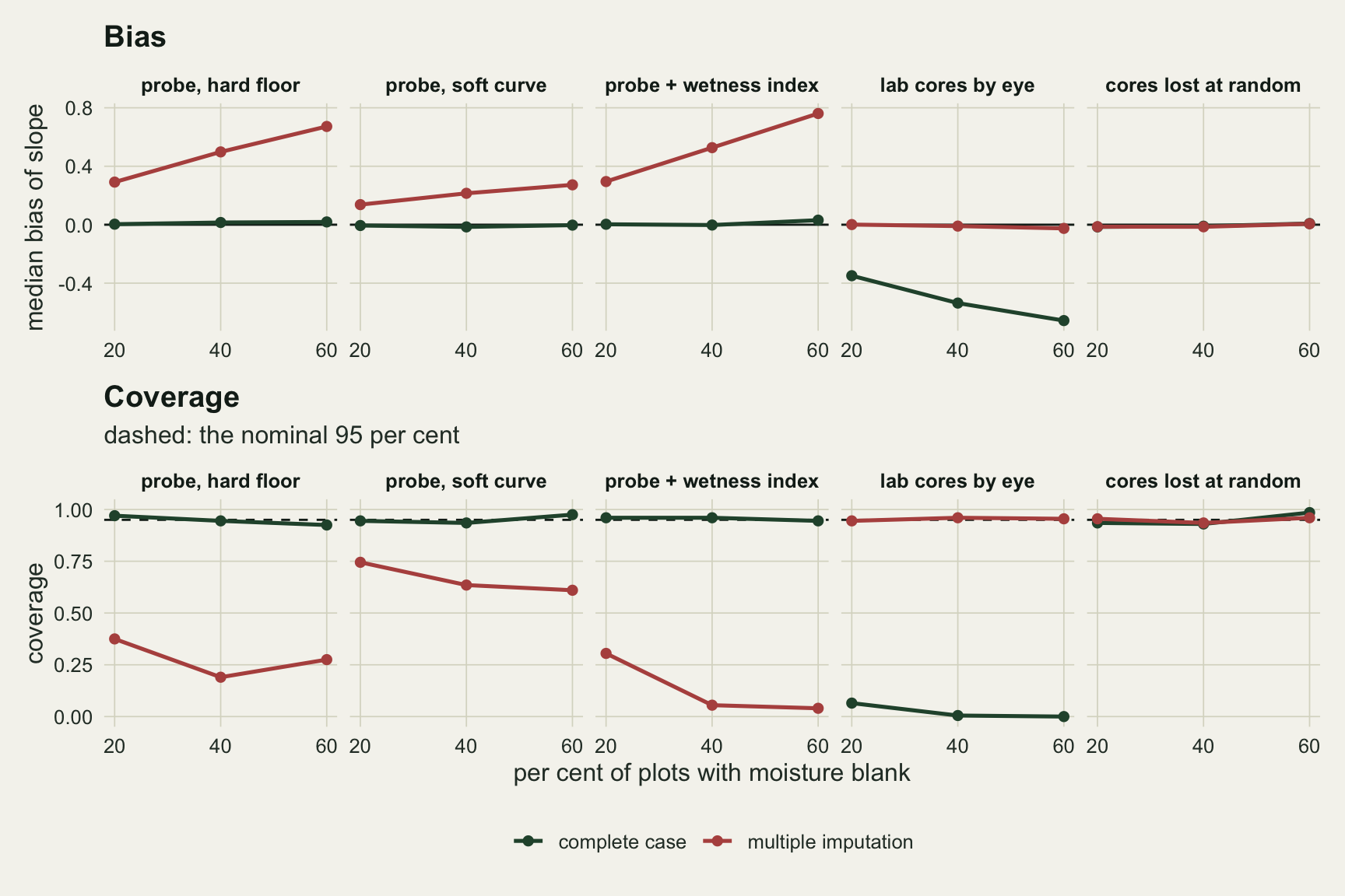
Neither the test nor the gap says which survey you are holding
If the reason decides the estimator, the reader needs to know the reason. The only thing the recorded data can test is whether the blanks are related to something recorded, and the obvious test is the one the assumption-checking post uses: a logistic regression of the missingness indicator on the observed variable, here glm(is.na(x) ~ y, family = binomial).
d_main <- all_draws[abs(all_draws$share - share_main) < 1e-9 &
                    all_draws$case %in% c("probe", "lab", "lost"), ]
gap_probe_q <- quantile(d_main$mi[d_main$case == "probe"] - d_main$cc[d_main$case == "probe"],
                        c(0.1, 0.9))
gap_lab_q <- quantile(d_main$mi[d_main$case == "lab"] - d_main$cc[d_main$case == "lab"],
                      c(0.1, 0.9))
At forty per cent blank the test rejects at the five per cent level in 200 of the 200 probe data sets and 200 of the 200 laboratory data sets, against 6 for the random losses, where its nominal rate would give about 10. It does what it is built to do: it separates both surveys from the lost box, which rules out random losses, the case where the choice matters least. It cannot separate the two surveys from each other, and the direction of the fitted effect does not help either: the coefficient of biomass in the test is negative, fewer blanks where biomass is high, in 200 of the probe data sets and 200 of the laboratory data sets. That is because in both the plots with a reading have more biomass than the plots without, in one case because the moisture that was read also drove the biomass and in the other because the biomass drove the reading.
The next thing to try is the disagreement between the two estimators themselves. Under random losses they agree, so a large gap says the blanks are not random. But the sign does not help: multiple imputation is above complete-case analysis in 200 of the 200 probe data sets, with a median gap of +0.495, and in 200 of the 200 laboratory data sets, with a median gap of +0.524. The central eighty per cent of gaps runs from +0.360 to +0.617 in the probe survey and from +0.428 to +0.639 in the laboratory survey. The two surveys produce the same diagnostic and the same disagreement in the same direction, and the right answer is at the bottom of the gap in one and at the top in the other.
d_main$survey <- factor(case_lab[d_main$case], levels = case_lab[c("probe", "lab", "lost")])
d_main$log_p <- -log10(pmax(d_main$p_diag, 1e-300))
p_diag_plot <- ggplot(d_main, aes(survey, log_p)) +
  geom_hline(yintercept = -log10(0.05), colour = te_ink, linetype = "dashed", linewidth = 0.5) +
  geom_jitter(width = 0.2, height = 0, size = 0.8, alpha = 0.6, colour = te_forest) +
  scale_y_sqrt() +
  labs(x = NULL, y = "-log10 p of the missingness test",
       title = "The test fires for both", subtitle = "square-root axis; dashed: p = 0.05") +
  theme_datasheet() + theme(axis.text.x = element_text(angle = 15, hjust = 1))
p_gap_plot <- ggplot(d_main, aes(survey, mi - cc)) +
  geom_hline(yintercept = 0, colour = te_ink, linewidth = 0.5) +
  geom_jitter(width = 0.2, height = 0, size = 0.8, alpha = 0.6, colour = te_rust) +
  labs(x = NULL, y = "imputation minus complete case",
       title = "The gap has the same sign", subtitle = "per data set") +
  theme_datasheet() + theme(axis.text.x = element_text(angle = 15, hjust = 1))
p_diag_plot + p_gap_plot + plot_annotation(theme = theme_datasheet())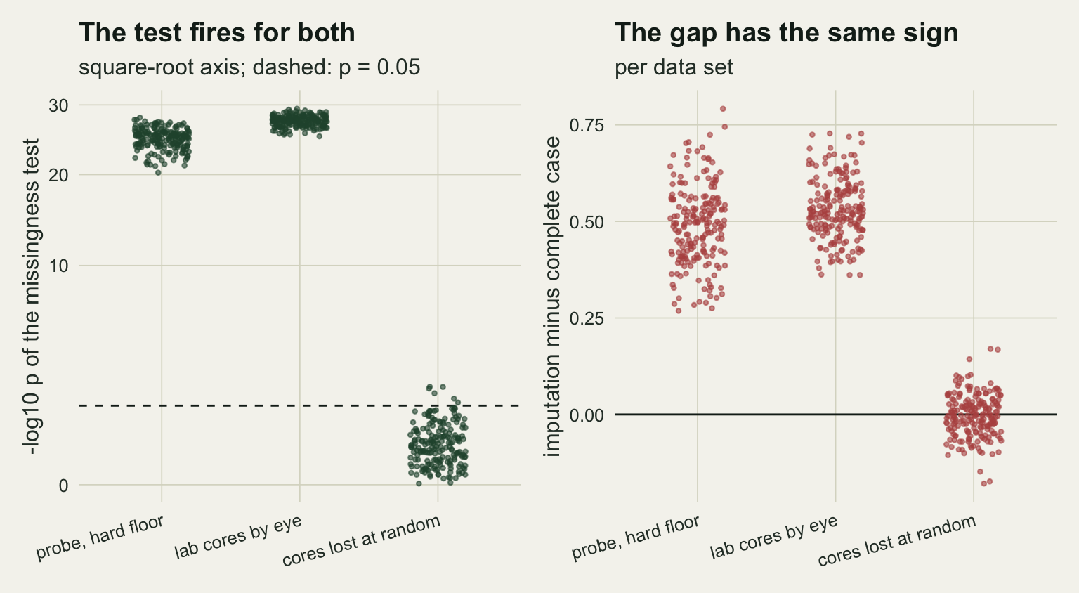
What to record and what to report
The measurement that settles the choice is not in the data frame, and no model fitted later recovers it. It is the reason the cell was left blank, and it is known to exactly one person at exactly one moment: whoever was standing at the plot when the reading did not happen. A reason-code column on the field sheet, filled in at that moment, costs a few characters per blank: probe would not enter, not cored, core lost, logger failed. With it the analysis becomes a lookup. Blanks caused by the value itself (a probe floor, a scale that tops out, or the detection limit of a laboratory assay moved to the predictor side) are a selection on the predictor, and deletion is safe for the slope. Blanks caused by something recorded, the response included, are what imputation is built for, provided that something is in the imputation model. Blanks caused by accident are harmless to both, and imputation is the more efficient of the two.
A floor in the observed values is a reason code the instrument writes for you. The hard probe floor leaves every recorded moisture above a sharp lower edge, and a histogram of the recorded values shows it; the soft failure curve leaves no edge, and neither does the laboratory selection.
Report the share of rows with the predictor blank, the reason, and how the reason was known: a field code, an instrument floor, or an argument. If the reason is not known, report both estimates, complete-case and multiple imputation, side by side, and say that the data cannot choose between them. The gap between them is then the honest width of what the missing reason code would have settled, and it belongs in the paper, not in a supplement.
Do not use the logistic missingness test as a licence for imputation. It rejected in the probe survey, where imputation is the wrong choice, as reliably as in the laboratory survey, where it is the right one. And do not fill a predictor with its fitted value from a regression on the response; that fill was wrong in all three surveys at forty per cent, the random losses included.
Nakagawa and Freckleton 2008 made the case to ecologists that deleting incomplete rows is not a neutral default, and it is not. The measurements here add the other half: imputing is not a neutral default either, and which one is the default depends on a fact that has to be written down at the plot.
Honest limits
The design is the friendliest one available: one predictor, a straight line, normal errors, five hundred plots, and an imputation model that is correctly specified whenever the mechanism allows it to be. With several predictors the condition for complete-case analysis is the same (the blank may depend on any of the predictors but not on the response given them), but a blank that depends on one predictor distorts the imputation of every other incomplete predictor that is imputed from it, and the size of the damage has to be measured again; White and Carlin 2010 is the place to start for those designs.
The laboratory selection is strong: the odds of coring a plot multiply by e for every unit of biomass, and biomass has a standard deviation of 2.83. A weaker selection on the response would give a smaller complete-case bias. The direction does not depend on the strength, but the numbers above do.
The imputation that fails in the probe survey is the one most people would build, imputing from the response under missing at random. It is not the only one. A model that knows about the floor, a truncated or censored model for moisture, can in principle impute below the floor correctly. That requires knowing where the floor is, which is again a reason code, and it is not demonstrated here.
Everything here is about the slope. The mean moisture of the survey area is a different target, and for it complete-case analysis is biased in the probe survey, since every dry plot is gone; a reader who wants a map of moisture from the same data is in a different problem.
The grid uses 200 data sets per cell, so a coverage near 0.95 carries a Monte Carlo standard error of about 0.015, and differences between cells smaller than two or three times that should not be read as real.
References
Little RJA 1992 Journal of the American Statistical Association 87(420):1227-1237 (10.1080/01621459.1992.10476282)
White IR, Carlin JB 2010 Statistics in Medicine 29(28):2920-2931 (10.1002/sim.3944)
Rubin DB 1976 Biometrika 63(3):581-592 (10.1093/biomet/63.3.581)
Barnard J, Rubin DB 1999 Biometrika 86(4):948-955 (10.1093/biomet/86.4.948)
Nakagawa S, Freckleton RP 2008 Trends in Ecology and Evolution 23(11):592-596 (10.1016/j.tree.2008.06.014)