library(ggplot2)
library(patchwork)

te_paper  <- "#f5f4ee"
te_ink    <- "#16241d"
te_body   <- "#2c3a31"
te_forest <- "#275139"
te_rust   <- "#b5534e"
te_gold   <- "#c9b458"
te_line   <- "#dad9ca"

theme_datasheet <- function() {
  theme_minimal(base_size = 12) +
    theme(plot.background  = element_rect(fill = te_paper, colour = NA),
          panel.background = element_rect(fill = te_paper, colour = NA),
          panel.grid.major = element_line(colour = te_line, linewidth = 0.3),
          panel.grid.minor = element_blank(),
          text             = element_text(colour = te_body),
          plot.title       = element_text(colour = te_ink, face = "bold"),
          plot.subtitle    = element_text(colour = te_body),
          axis.text        = element_text(colour = te_body))
}Interpolated cores and false slowing down
R
early warning signals
palaeoecology
time series
resilience
simulation
ecology tutorial
Interpolating an unevenly sampled core to a regular grid can fake or hide critical slowing down. In R: when it happens, why, and a null that corrects the test.
A lake core has been sliced at one centimetre, dated at a handful of levels and run through an age-depth model. The diatom-inferred proxy shows an abrupt shift near the top, and the question is whether the lake announced it: did the proxy slow down, in the sense of critical slowing down, before the shift? The early warning toolbox wants a regular clock, so the slices are linearly interpolated onto a ten-year grid, a rolling lag-1 autocorrelation is computed over half the record, its trend is summarised by Kendall’s tau, and the tau is tested against surrogate series. The slices, though, were never ten years apart. The years per centimetre changed with accumulation and compaction, and so the gap between neighbouring samples drifts along the core.
That drift decides the answer before any indicator is computed. A grid point that falls inside a long gap between two samples is a weighted mean of those two samples, and so is its neighbour on the grid; the longer the gap, the more often two adjacent grid points are built from the same samples, and the more alike they are. When the spacing coarsens toward the event, the indicator rises with nothing happening. When the spacing refines toward it, as compaction tends to make it toward the young end of a core, a real rise is flattened. How much of either happens depends on how much memory the proxy itself has at the grid step: a proxy that is nearly uncorrelated from one decade to the next leaves the whole lag-1 structure of the grid to the interpolation, a persistent one leaves the interpolation less to add.
The early warning posts on this site all work on a regular clock. Early warning signals and critical slowing samples its fold “at unit intervals, as an annual monitoring record would be”, and Checking early warning signals builds a version of the surrogate test used here and measures how often the naive and surrogate tests cry wolf, again on regularly spaced series; its example of a warning without a transition comes from noise that grows through the record. Detrending and bandwidth in early warning signals varies the analyst’s choices on the same regular series. Uneven spacing appears in two core posts: Age-depth models and what they do to a proxy interpolates the age axis and follows dating error into influx, and Pollen rate of change and uneven sample spacing shows that dividing by the gap puts the rate-of-change peaks on the shortest gaps. Neither computes an early warning indicator. The repair used below has the logic of Tuning proxy records manufactures synchrony, whose null is tuned the same way as the data.
None of the parts is new. Rehfeld and colleagues showed in 2011 that interpolating an irregularly sampled series strongly overestimates its persistence. Dakos and colleagues warned in their 2012 methods paper that interpolation can produce spurious correlations and that the density of interpolated points should be checked to be constant along the record, and in 2008 they checked their own palaeoclimate results by recomputing autocorrelation on the non-interpolated data. Braun and colleagues built surrogates that respect the sampling for recurrence analysis of irregular records in 2022, and found a spurious transition caused only by a shift in sampling rate. Ben-Yami and colleagues showed in 2023 that non-stationary data coverage, together with the gap filling used to deal with it, can give a false indication of critical slowing down in sea-surface temperature and salinity records, and built surrogate tests that account for the coverage. So the false alarm itself is known. What this post adds, for the test people run on a core, is the other direction (spacing that refines toward the event hides a real rise), how both directions depend on the proxy’s own memory at the grid step, and what the check on the non-interpolated samples does in each case. It also measures, in one simple setting, how often the standard surrogate test flags a record with no transition and how much of the damage a null that goes through the same interpolation removes. The rise of the indicator itself is closed form, and it is derived below rather than presented as a finding.
A core on an uneven clock
The proxy is an annual AR(1) process with unit variance and lag-1 coefficient \(\phi\), so its true autocorrelation at the ten-year grid step is \(\phi^{10}\). Each record covers 2000 years. Sample ages are built one at a time: the next gap is the local target spacing, which runs linearly from \(d_0\) years at the old end to \(d_1\) at the young end, times a uniform jitter of plus or minus 30 per cent, rounded to whole years. The samples are interpolated linearly onto a ten-year grid, the lag-1 autocorrelation is computed in a rolling window of half the gridded series, and the indicator’s trend is Kendall’s tau against time.
Two tests are applied to every record. The standard test fits an AR(1) model to the gridded series and simulates 49 surrogate series of the same length on the grid; the p-value is \((1 + k)/(B + 1)\), where \(k\) of the \(B = 49\) surrogate taus are at least the observed one, and the record is flagged when it is at most 0.05. The pipeline test fits a continuous-time AR(1) (Ornstein-Uhlenbeck) process to the raw samples by its exact likelihood at the real ages, from three starting values of its time scale, simulates 49 surrogates at those same ages, and pushes each one through the same interpolation and the same rolling window. Because an annual AR(1) is an Ornstein-Uhlenbeck process observed at whole years, the pipeline null is correctly specified here by construction; that is a choice of the demonstration, and it comes back in the limits.
t_len <- 2000; grid_step <- 10; jit <- 0.3; n_sur <- 49; alpha <- 0.05

kendall_tau <- function(M) {                # Kendall tau of each column against its index
  M <- as.matrix(M); n <- nrow(M)
  ij <- which(upper.tri(diag(n)), arr.ind = TRUE)
  colSums(sign(M[ij[, 2], , drop = FALSE] - M[ij[, 1], , drop = FALSE])) / nrow(ij)
}
roll_ac1 <- function(Y, w) {                # rolling lag-1 correlation, one column per series
  Y <- as.matrix(Y); n <- nrow(Y)
  A <- Y[-n, , drop = FALSE]; Bm <- Y[-1, , drop = FALSE]
  cz <- function(M) rbind(0, apply(M, 2, cumsum))
  ca <- cz(A); cb <- cz(Bm); caa <- cz(A * A); cbb <- cz(Bm * Bm); cab <- cz(A * Bm)
  k <- w - 1; i <- 1:(n - w + 1); j <- i + k
  sa <- ca[j, , drop = FALSE] - ca[i, , drop = FALSE]
  sb <- cb[j, , drop = FALSE] - cb[i, , drop = FALSE]
  vaa <- caa[j, , drop = FALSE] - caa[i, , drop = FALSE] - sa^2 / k
  vbb <- cbb[j, , drop = FALSE] - cbb[i, , drop = FALSE] - sb^2 / k
  vab <- cab[j, , drop = FALSE] - cab[i, , drop = FALSE] - sa * sb / k
  vab / sqrt(vaa * vbb)
}
roll_var <- function(y, w) {
  n <- length(y); cs <- c(0, cumsum(y)); cq <- c(0, cumsum(y * y))
  i <- 1:(n - w + 1); j <- i + w; s <- cs[j] - cs[i]
  (cq[j] - cq[i] - s^2 / w) / (w - 1)
}
sim_ages <- function(d0, d1) {
  a <- 1; ages <- a
  repeat {
    d <- d0 + (d1 - d0) * (a / t_len)
    a <- a + max(1, round(d * runif(1, 1 - jit, 1 + jit)))
    if (a > t_len) break
    ages <- c(ages, a)
  }
  ages
}
sim_proxy <- function(phi_path) {           # annual AR(1), unit variance at every step
  x <- numeric(t_len); x[1] <- rnorm(1); e <- rnorm(t_len)
  for (i in 2:t_len) x[i] <- phi_path[i] * x[i - 1] + sqrt(1 - phi_path[i]^2) * e[i]
  x
}
interp_weights <- function(ages, g) {       # linear interpolation written as a weight matrix
  W <- matrix(0, length(g), length(ages))
  k <- findInterval(g, ages, rightmost.closed = TRUE)
  k[k == length(ages)] <- length(ages) - 1
  wr <- (g - ages[k]) / (ages[k + 1] - ages[k])
  W[cbind(seq_along(g), k)] <- 1 - wr; W[cbind(seq_along(g), k + 1)] <- wr
  W
}
ou_negll <- function(p, tt, x) {            # exact Ornstein-Uhlenbeck likelihood at irregular times
  mu <- p[1]; s <- exp(p[2]); r <- exp(-diff(tt) / exp(p[3]))
  m <- mu + r * (x[-length(x)] - mu); v <- s^2 * (1 - r^2)
  -(dnorm(x[1], mu, s, log = TRUE) + sum(dnorm(x[-1], m, sqrt(v), log = TRUE)))
}
fit_ou <- function(tt, x) {
  best <- NULL
  for (tau0 in c(2, 10, 50)) {
    f <- optim(c(mean(x), log(sd(x)), log(tau0)), ou_negll, tt = tt, x = x, method = "BFGS")
    if (is.null(best) || f$value < best$value) best <- f
  }
  c(mu = best$par[1], s = exp(best$par[2]), tau = exp(best$par[3]))
}
sim_ou <- function(tt, fo, B) {             # B Ornstein-Uhlenbeck paths at the real ages
  X <- matrix(0, length(tt), B); X[1, ] <- rnorm(B, fo["mu"], fo["s"])
  r <- exp(-diff(tt) / fo["tau"])
  for (k in 2:length(tt))
    X[k, ] <- fo["mu"] + r[k - 1] * (X[k - 1, ] - fo["mu"]) + rnorm(B, 0, fo["s"] * sqrt(1 - r[k - 1]^2))
  X
}
sim_ar1_grid <- function(phi, sdv, n, B) {  # B stationary AR(1) surrogates on the grid
  E <- matrix(rnorm(n * B, 0, sdv), n, B); E[1, ] <- rnorm(B, 0, sdv / sqrt(1 - phi^2))
  for (k in 2:n) E[k, ] <- phi * E[k - 1, ] + E[k, ]
  E
}
gauss_detrend <- function(y, bw) {
  tg <- seq_along(y); K <- outer(tg, tg, function(a, b) dnorm(a, b, bw))
  y - as.numeric((K / rowSums(K)) %*% y)
}
std_test <- function(y, w, tau_obs) {       # AR(1) fitted to the gridded series
  a1 <- ar.ols(y, order.max = 1, aic = FALSE, demean = TRUE)
  ph <- max(min(a1$ar[1], 0.99), -0.99)
  ts <- kendall_tau(roll_ac1(sim_ar1_grid(ph, sqrt(a1$var.pred), length(y), n_sur), w))
  (1 + sum(ts >= tau_obs)) / (n_sur + 1)
}
one_record <- function(phi_path, d0, d1, step = grid_step) {
  x <- sim_proxy(phi_path); ages <- sim_ages(d0, d1); xs <- x[ages]
  g <- seq(ceiling(min(ages) / step) * step, max(ages), by = step)
  W <- interp_weights(ages, g); yg <- as.numeric(W %*% xs); w <- floor(length(yg) / 2)
  tau_obs <- kendall_tau(roll_ac1(yg, w))
  rd <- gauss_detrend(yg, 0.1 * length(yg)); tau_dt <- kendall_tau(roll_ac1(rd, w))
  fo <- fit_ou(ages, xs)
  ts_pipe <- kendall_tau(roll_ac1(W %*% sim_ou(ages, fo, n_sur), w))
  c(tau = tau_obs, tau_raw = kendall_tau(roll_ac1(xs, floor(length(xs) / 2))),
    tau_var = kendall_tau(roll_var(yg, w)), tau_dt = tau_dt,
    p_std = std_test(yg, w, tau_obs), p_dt = std_test(rd, w, tau_dt),
    p_pipe = (1 + sum(ts_pipe >= tau_obs)) / (n_sur + 1),
    n_samp = length(xs), ou_scale = unname(fo["tau"]))
}
run_cell <- function(n_rec, phi0, phi1, d0, d1, step = grid_step) {
  pp <- seq(phi0, phi1, length.out = t_len)
  as.data.frame(t(replicate(n_rec, one_record(pp, d0, d1, step))))
}
mcse <- function(p, n) sqrt(p * (1 - p) / n)
set.seed(33000)
tau_check <- matrix(rnorm(300), 100, 3)
gap_kendall <- max(abs(kendall_tau(tau_check) - cor(1:100, tau_check, method = "kendall")))
The Kendall tau is computed by counting concordant pairs directly, which is faster inside the loops than cor(); on a test matrix the two agree to machine precision.
The first picture is one proxy record sampled twice. The annual series is the same; only the sampling differs. In one version the gaps grow from 4 to 16 years toward the young end, in the other they shrink from 16 to 4.
phi_base <- 0.9; phi_top <- 0.99
set.seed(33010)
x_ex <- sim_proxy(rep(phi_base, t_len))
ex_one <- function(d0, d1, label) {
  ages <- sim_ages(d0, d1); g <- seq(ceiling(min(ages) / grid_step) * grid_step, max(ages), by = grid_step)
  yg <- as.numeric(interp_weights(ages, g) %*% x_ex[ages]); w <- floor(length(yg) / 2)
  ac <- as.numeric(roll_ac1(yg, w))
  list(gaps = data.frame(age = ages[-1], gap = diff(ages), design = label),
       ac = data.frame(age = g[w:length(g)], ac1 = ac, design = label),
       tau = kendall_tau(ac))
}
ex_c <- ex_one(4, 16, "coarsening 4 to 16 yr")
ex_r <- ex_one(16, 4, "refining 16 to 4 yr")
The coarsening version gives a Kendall tau of 0.71, the refining version -0.51, from the same annual values, whose true ten-year autocorrelation is 0.349 everywhere.
ex_cols <- c("coarsening 4 to 16 yr" = te_rust, "refining 16 to 4 yr" = te_forest)
p_gap <- ggplot(rbind(ex_c$gaps, ex_r$gaps), aes(age, gap, colour = design)) +
  geom_point(size = 0.9, alpha = 0.7) +
  scale_colour_manual(values = ex_cols, name = NULL) +
  labs(x = "sample age (yr from the old end)", y = "gap to previous sample (yr)",
       title = "The sampling") +
  theme_datasheet() + theme(legend.position = "none")
p_ac <- ggplot(rbind(ex_c$ac, ex_r$ac), aes(age, ac1, colour = design)) +
  geom_hline(yintercept = phi_base^10, colour = te_ink, linetype = "dashed", linewidth = 0.5) +
  geom_line(linewidth = 0.9) +
  annotate("text", x = 1000, y = phi_base^10, label = "true 10-yr autocorrelation",
           hjust = 0, vjust = -0.6, colour = te_ink, size = 3.3) +
  scale_colour_manual(values = ex_cols, name = NULL) +
  labs(x = "end of window (years)", y = "rolling lag-1 autocorrelation",
       title = "The indicator") +
  theme_datasheet() + theme(legend.position = "bottom")
p_gap + p_ac + plot_layout(guides = "collect") +
  plot_annotation(theme = theme_datasheet() + theme(legend.position = "bottom"))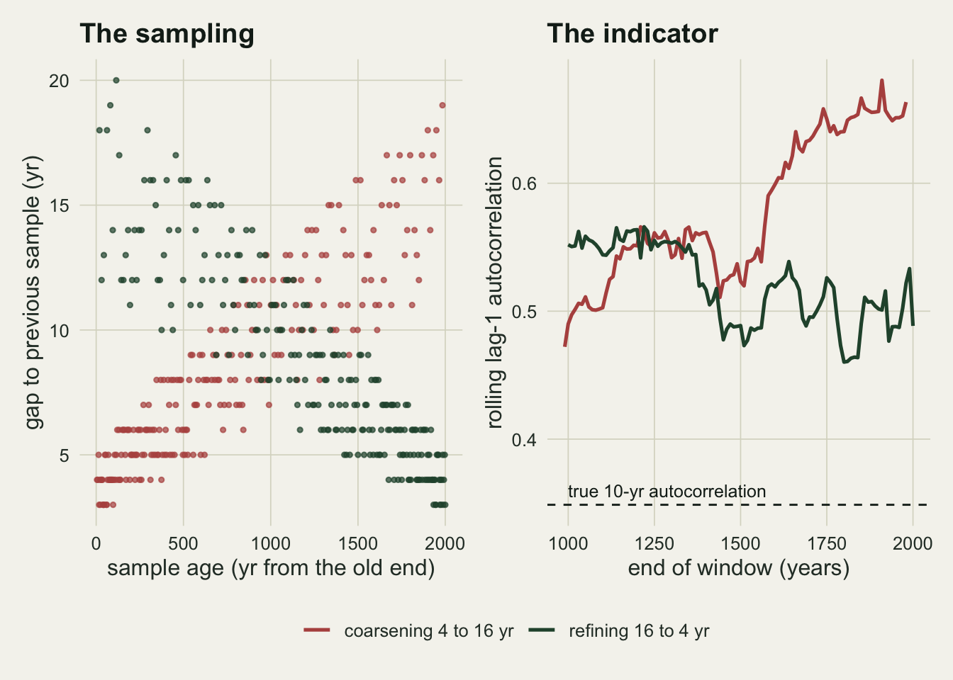
Two ways to be wrong
The main simulation holds the proxy’s memory at \(\phi = 0.90\), a ten-year autocorrelation of 0.35, and crosses five spacing designs with two truths. Without a transition, \(\phi\) stays at 0.90 for the whole record, and a flag is a false alarm. With a real slowing, \(\phi\) rises linearly from 0.90 to 0.99 across the record (the ten-year autocorrelation from 0.35 to 0.90) with the variance held at one, so only the memory changes, and a flag is a detection. The replication, 250 records per cell, was fixed before any rate was looked at.
designs <- data.frame(
  name = c("even 10", "coarsening 4 to 16", "refining 16 to 4", "mild coarsening 8 to 12", "mild refining 12 to 8"),
  d0 = c(10, 4, 16, 8, 12), d1 = c(10, 16, 4, 12, 8))
n_table <- 250
set.seed(33020)
cells_null <- lapply(seq_len(nrow(designs)), function(i)
  run_cell(n_table, phi_base, phi_base, designs$d0[i], designs$d1[i]))
cells_slow <- lapply(seq_len(nrow(designs)), function(i)
  run_cell(n_table, phi_base, phi_top, designs$d0[i], designs$d1[i]))
names(cells_null) <- names(cells_slow) <- designs$name
flag <- function(r, col = "p_std") mean(r[[col]] <= alpha)
dec <- do.call(rbind, lapply(designs$name, function(nm) data.frame(
  design = nm,
  truth = rep(c("no transition", "real slowing"), each = 2),
  test = rep(c("standard AR(1) surrogates", "pipeline null"), 2),
  rate = c(flag(cells_null[[nm]]), flag(cells_null[[nm]], "p_pipe"),
           flag(cells_slow[[nm]]), flag(cells_slow[[nm]], "p_pipe")))))
dec$se <- mcse(dec$rate, n_table)
rate_of <- function(nm, truth, test) dec$rate[dec$design == nm & dec$truth == truth & dec$test == test]
std_lab <- "standard AR(1) surrogates"; pipe_lab <- "pipeline null"
mask_drop <- rate_of("even 10", "real slowing", std_lab) - rate_of("refining 16 to 4", "real slowing", std_lab)
pipe_null_max <- max(dec$rate[dec$truth == "no transition" & dec$test == pipe_lab])
n_samp_med <- median(unlist(lapply(cells_null, function(r) r$n_samp)))
The records carry a median of 205 samples. On even spacing the standard test is, if anything, conservative: it flags 0.024 of the records without a transition (Monte Carlo standard error 0.010) and detects the real slowing in 0.456. With spacing that coarsens from 4 to 16 years it flags 0.288 of the records without a transition, and a mild drift from 8 to 12 years gives 0.084. Running the other way, spacing that refines from 16 to 4 years detects the real slowing in 0.128 of the records, a loss of 0.328 against even spacing; the mild refining drift gives 0.372. On the null records the refining designs flag 0.004 and 0.008: the test has become conservative, which is the same effect seen from the other side.
The pipeline null flags between 0.016 and 0.068 of the records without a transition in all five designs. Its power is 0.500 on even spacing, 0.464 with refining spacing and 0.364 with coarsening spacing. The standard test’s 0.744 in that last cell is not power: it is the false alarm added to the real rise.
dec$design <- factor(dec$design, levels = rev(designs$name))
dec$test <- factor(dec$test, levels = c(std_lab, pipe_lab))
p_table <- ggplot(dec, aes(rate, design, colour = test)) +
  geom_vline(data = data.frame(truth = "no transition", x = alpha), aes(xintercept = x),
             colour = te_body, linetype = "dashed", linewidth = 0.4) +
  geom_errorbar(aes(xmin = pmax(rate - 2 * se, 0), xmax = rate + 2 * se), orientation = "y",
                width = 0.25, linewidth = 0.4, position = position_dodge(width = 0.5)) +
  geom_point(size = 2.6, position = position_dodge(width = 0.5)) +
  facet_wrap(~ truth, labeller = labeller(truth = c("no transition" = "No transition: false alarms",
                                                    "real slowing" = "Real slowing: detections"))) +
  scale_colour_manual(values = c(te_rust, te_forest), name = NULL) +
  scale_x_continuous(limits = c(0, 1), breaks = c(0, 0.25, 0.5, 0.75, 1),
                     labels = c("0", "0.25", "0.5", "0.75", "1")) +
  labs(x = "share of records flagged at p <= 0.05", y = NULL,
       title = "The spacing trend fakes a warning or hides one") +
  theme_datasheet() +
  theme(legend.position = "bottom", panel.spacing = unit(1.6, "lines"),
        strip.text = element_text(colour = te_ink, face = "bold"))
p_table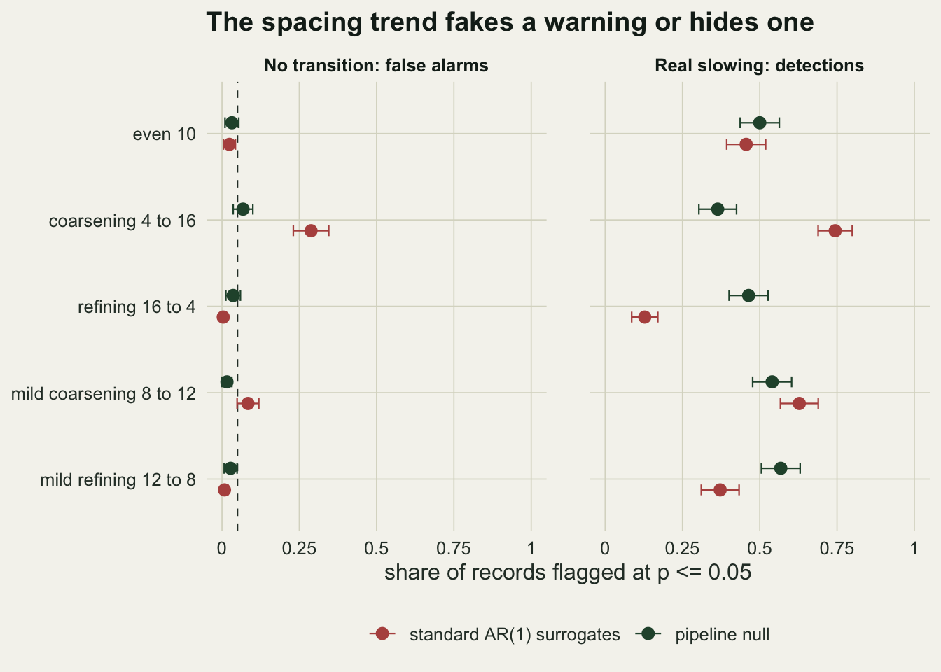
Why an interpolated grid remembers the gap
The rise of the indicator is algebra. Take regular sampling every \(D\) years and a grid point at time \(t\) that lies a fraction \(\lambda\) of the way from the sample at \(a\) to the sample at \(a + D\). Linear interpolation gives \(y(t) = (1 - \lambda)\,x(a) + \lambda\,x(a + D)\), and with the proxy’s autocorrelation \(\rho(h) = \phi^{|h|}\),
\[ \operatorname{Var} y(t) = (1-\lambda)^2 + \lambda^2 + 2\lambda(1-\lambda)\,\phi^{D}, \qquad \operatorname{Cov}\{y(t), y(t+10)\} = \sum_{i}\sum_{j} c_i\,c'_j\,\phi^{|s_i - s'_j|}, \]
where \(c_i\) and \(s_i\) are the two weights and sample ages behind \(y(t)\), and \(c'_j\), \(s'_j\) those behind \(y(t + 10)\). With whole-year ages and a random start, the offset of a grid point from the sample on its left is equally likely to be any of \(0, 1, \ldots, D - 1\) years, and the lag-1 autocorrelation of a long gridded series is the average covariance over those offsets divided by the average variance. When \(D\) is at most half the grid step, adjacent grid points are built from different samples, and only the smoothing inside each gap lifts their correlation above the proxy’s own \(\phi^{10}\). Between half the grid step and the grid step they can share one sample. Beyond the grid step many adjacent grid points share both samples, and their covariance approaches their variance.
ac1_closed <- function(phi, D, step = grid_step) {
  num <- 0; den <- 0
  for (u in 0:(D - 1)) {                       # offset of the grid point from the sample on its left
    c1 <- c(1 - u / D, u / D); s1 <- c(0, D)
    k2 <- floor((u + step) / D); l2 <- (u + step) / D - k2
    c2 <- c(1 - l2, l2); s2 <- c(k2 * D, (k2 + 1) * D)
    num <- num + sum(outer(c1, c2) * phi^abs(outer(s1, s2, "-")))
    den <- den + sum(outer(c1, c1) * phi^abs(outer(s1, s1, "-")))
  }
  num / den
}
phi_cf <- c(0.6, 0.9, 0.97); d_cf <- seq(4, 16, by = 2)
cf_tab <- expand.grid(D = d_cf, phi = phi_cf)
cf_tab$closed <- mapply(ac1_closed, cf_tab$phi, cf_tab$D)
pooled_ac1 <- function(phi, D, n_target = 80) {  # regular sampling, every start offset equally often
  n_each <- ceiling(n_target / D); sxy <- sxx <- numeric(n_each * D)
  for (r in seq_len(n_each * D)) {
    x <- sim_proxy(rep(phi, t_len)); ages <- seq((r - 1) %% D + 1, t_len, by = D)
    g <- seq(ceiling(min(ages) / grid_step) * grid_step, max(ages), by = grid_step)
    y <- as.numeric(interp_weights(ages, g) %*% x[ages]); n <- length(y)
    sxy[r] <- sum(y[-1] * y[-n]); sxx[r] <- sum(y[-n]^2)
  }
  est <- sum(sxy) / sum(sxx)                     # pooled ratio, and its delta-method standard error
  c(est = est, se = sqrt(sum((sxy - est * sxx)^2)) / sum(sxx))
}
set.seed(33030)
cf_sim <- t(mapply(pooled_ac1, cf_tab$phi, cf_tab$D))
cf_tab$simulated <- cf_sim[, "est"]; cf_tab$sim_se <- cf_sim[, "se"]
cf_gap <- max(abs(cf_tab$closed - cf_tab$simulated))
cf_z <- max(abs(cf_tab$closed - cf_tab$simulated) / cf_tab$sim_se)
cf_rise <- sapply(phi_cf, function(p) ac1_closed(p, 16) - ac1_closed(p, 4))
cf_at <- function(p, D) cf_tab$closed[cf_tab$phi == p & cf_tab$D == D]
Over three values of \(\phi\) and seven spacings, the closed form and the pooled lag-1 autocorrelation of at least 80 simulated records per cell, with every start offset used equally often, differ by at most 0.012, which is 2.1 Monte Carlo standard errors of the pooled estimate at most. At \(\phi = 0.6\), whose true ten-year autocorrelation is 0.006, the gridded series has a lag-1 autocorrelation of 0.015 with 4-year spacing and 0.596 with 16-year spacing. Across the same change in spacing the rise is 0.289 at \(\phi = 0.9\) and 0.103 at \(\phi = 0.97\). So a spacing trend is a trend in the indicator’s expected value, of a size fixed by \(\phi\) and the two spacings, and the standard surrogate, a stationary AR(1) on the grid, carries neither the spacing nor its trend.
The same algebra says what the raw samples do. Two neighbouring samples \(D\) years apart correlate at \(\phi^{D}\), which falls as the gap grows: 0.656 at 4 years and 0.185 at 16 years for \(\phi = 0.9\). With no change in the proxy, an indicator computed on the samples in their index order therefore moves the opposite way to the gridded one. That is the subject of the next section but one.
cf_tab$memory <- factor(sprintf("phi %.2f (10-yr AC %.2f)", cf_tab$phi, cf_tab$phi^10))
truth_lines <- data.frame(memory = levels(cf_tab$memory), y = sort(phi_cf)^10)
mem_cols <- setNames(c(te_rust, te_gold, te_forest), levels(cf_tab$memory))
ggplot(cf_tab, aes(D, closed, colour = memory)) +
  geom_hline(data = truth_lines, aes(yintercept = y, colour = memory), linetype = "dotted", linewidth = 0.6) +
  geom_line(linewidth = 1) +
  geom_point(aes(y = simulated), size = 2.4, shape = 21, fill = te_paper, stroke = 1) +
  scale_colour_manual(values = mem_cols, name = NULL) +
  scale_x_continuous(breaks = d_cf) + scale_y_continuous(limits = c(0, 1)) +
  labs(x = "years between samples", y = "lag-1 autocorrelation on the 10-yr grid",
       title = "The grid's memory grows with the gap") +
  guides(colour = guide_legend(nrow = 3)) +
  theme_datasheet() + theme(legend.position = "bottom")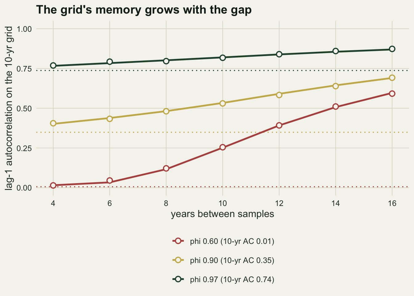
The closed form covers regular spacing and says nothing about jitter, the rolling window or the test. The false-alarm rate needs the null distribution of Kendall’s tau for an overlapping rolling indicator, which is wide (the checking post measures that width), and that is what the simulations are for.
The proxy’s own memory sets the size
The decision table fixed \(\phi\) at 0.90. The size of the artefact is the gap between the correlation the grid manufactures and the correlation the proxy already has at the grid step, so the rate should fall as the proxy’s memory rises. The cells below repeat the two coarsening designs without a transition at four more values of \(\phi\), 300 records per cell for the strong drift and 150 for the mild one; the \(\phi = 0.90\) cells come from the table.
phi_grid <- c(0.6, 0.8, 0.95, 0.97); n_phi <- 300; n_phi_mild <- 150
set.seed(33040)
phi_cells <- lapply(phi_grid, function(p) list(
  strong = run_cell(n_phi, p, p, 4, 16), mild = run_cell(n_phi_mild, p, p, 8, 12)))
phi_curve <- rbind(
  do.call(rbind, lapply(seq_along(phi_grid), function(i) data.frame(
    phi = phi_grid[i], design = c("coarsening 4 to 16", "mild coarsening 8 to 12"),
    std = c(flag(phi_cells[[i]]$strong), flag(phi_cells[[i]]$mild)),
    pipe = c(flag(phi_cells[[i]]$strong, "p_pipe"), flag(phi_cells[[i]]$mild, "p_pipe")),
    tau = c(median(phi_cells[[i]]$strong$tau), median(phi_cells[[i]]$mild$tau)), n = c(n_phi, n_phi_mild)))),
  data.frame(phi = phi_base, design = c("coarsening 4 to 16", "mild coarsening 8 to 12"),
             std = c(flag(cells_null[["coarsening 4 to 16"]]), flag(cells_null[["mild coarsening 8 to 12"]])),
             pipe = c(flag(cells_null[["coarsening 4 to 16"]], "p_pipe"),
                      flag(cells_null[["mild coarsening 8 to 12"]], "p_pipe")),
             tau = c(median(cells_null[["coarsening 4 to 16"]]$tau),
                     median(cells_null[["mild coarsening 8 to 12"]]$tau)), n = n_table))
phi_curve <- phi_curve[order(phi_curve$design, phi_curve$phi), ]
phi_curve$ac10 <- phi_curve$phi^10
pc <- function(p, dsg, col = "std") phi_curve[[col]][phi_curve$phi == p & phi_curve$design == dsg]
pipe_phi_max <- max(phi_curve$pipe)
With the strong drift the standard test flags 0.610 of the records when the proxy is nearly uncorrelated at the grid step (\(\phi = 0.6\), standard error 0.028), 0.487 at \(\phi = 0.8\) (ten-year autocorrelation 0.11), 0.288 at 0.9, 0.217 at 0.95 and 0.150 at 0.97 (ten-year autocorrelation 0.74). The rate falls across the whole range and is still well above nominal at the most persistent proxy tried (standard error 0.021 at \(\phi = 0.97\)). The mild drift gives 0.140 at \(\phi = 0.6\) and 0.047 at 0.97. The pipeline null stays at or below 0.068 in every one of these cells.
phi_long <- rbind(data.frame(phi_curve[, c("ac10", "design", "n")], test = std_lab, rate = phi_curve$std),
                  data.frame(phi_curve[, c("ac10", "design", "n")], test = pipe_lab, rate = phi_curve$pipe))
phi_long$se <- mcse(phi_long$rate, phi_long$n)
phi_long$test <- factor(phi_long$test, levels = c(std_lab, pipe_lab))
ggplot(phi_long, aes(ac10, rate, colour = test, linetype = design)) +
  geom_hline(yintercept = alpha, colour = te_body, linetype = "dashed", linewidth = 0.4) +
  geom_errorbar(aes(ymin = pmax(rate - 2 * se, 0), ymax = rate + 2 * se), width = 0.015,
                linewidth = 0.4, linetype = "solid") +
  geom_line(linewidth = 0.9) + geom_point(size = 2.2) +
  scale_colour_manual(values = c(te_rust, te_forest), name = NULL) +
  scale_linetype_manual(values = c("solid", "longdash"), name = NULL) +
  scale_y_continuous(limits = c(0, 1)) +
  labs(x = "proxy's own autocorrelation at the 10-yr grid step", y = "false-alarm rate",
       title = "The more memory the proxy has, the less the grid adds") +
  guides(colour = guide_legend(nrow = 2), linetype = guide_legend(nrow = 2)) +
  theme_datasheet() + theme(legend.position = "bottom", legend.key.width = unit(2.6, "lines"))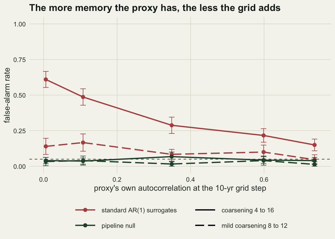
The check on the raw samples has its own artefact
Dakos and colleagues checked their 2008 result by recomputing autocorrelation on the non-interpolated data, and reported approximately similar results. The rolling lag-1 autocorrelation of the raw samples in their index order is that check. Under a spacing trend it carries its own artefact, of the opposite sign, because the correlation between neighbouring samples is \(\phi^{D}\). The rolling variance of the gridded series is the other cross-check people reach for, since critical slowing down should raise variance with autocorrelation.
raw_long <- do.call(rbind, lapply(c("even 10", "coarsening 4 to 16", "refining 16 to 4"), function(nm) rbind(
  data.frame(design = nm, truth = "no transition", tau = cells_null[[nm]]$tau, tau_raw = cells_null[[nm]]$tau_raw),
  data.frame(design = nm, truth = "real slowing", tau = cells_slow[[nm]]$tau, tau_raw = cells_slow[[nm]]$tau_raw))))
med_of <- function(cells, nm, col) median(cells[[nm]][[col]])
opp_sign <- function(nm) mean(sign(cells_null[[nm]]$tau) != sign(cells_null[[nm]]$tau_raw))
dt_gap <- max(abs(sapply(designs$name, function(nm) flag(cells_null[[nm]], "p_dt") - flag(cells_null[[nm]]))))
conj <- function(r) mean(r$p_std <= alpha & r$tau_raw > 0)   # gridded flag confirmed by a rising raw indicator
conj_phi <- function(p) conj(phi_cells[[which(phi_grid == p)]]$strong)
flag_phi <- function(p) flag(phi_cells[[which(phi_grid == p)]]$strong)
raw_up_null_ref <- mean(cells_null[["refining 16 to 4"]]$tau_raw > 0)
sc <- cells_slow[["coarsening 4 to 16"]]
veto_both <- mean(sc$p_std <= alpha & sc$p_pipe <= alpha & sc$tau_raw <= 0)   # flagged by both tests, vetoed
Without a transition and with coarsening spacing, the gridded indicator has a median tau of +0.66 and the raw-sample indicator -0.77; with refining spacing the two are -0.65 and +0.72. The signs disagree in 0.888 and 0.852 of those records. On even spacing the two medians are -0.03 and -0.03. With a real slowing and even spacing they are +0.76 and +0.78; with a real slowing and refining spacing the gridded median falls to +0.54 while the raw one is +0.92, so both still rise; with a real slowing and coarsening spacing the raw one is -0.03, as if nothing were changing.
So the raw-sample indicator is not a neutral check: it carries the mirror image of the grid’s artefact. Used the way the 2008 check was used, accepting a gridded warning only if the raw indicator also rises, it cuts the standard test’s false alarms with strong coarsening from 0.288 to 0.020 at \(\phi = 0.90\). It does so only because its own artefact runs the other way, and that artefact needs memory between neighbouring samples: at \(\phi = 0.6\), where two samples 4 years apart correlate at 0.13 and samples 16 years apart at almost nothing, the combined rule still flags 0.263 of the null records with strong coarsening, against 0.610 for the standard test alone. With the mild drift at \(\phi = 0.90\) it removes little: 0.068 against 0.084. With a real slowing and coarsening spacing it cuts the detections from 0.744 to 0.416; part of what it removes is the false alarm riding on the real rise, but not all of it: the pipeline null detects 0.364 in the same cell, and 0.124 of the records are flagged by both tests and still vetoed by the rule. Under refining spacing the rule can only remove flags, so it cannot bring back the warnings the grid has flattened: 0.128 of the real slowings pass it, against 0.128 for the standard test alone.
The chunk below tests the raw-sample indicator on its own, with the same standard surrogates fitted to the samples in their index order, on records without a transition, 250 per design.
raw_p <- function(d0, d1) {
  xs <- sim_proxy(rep(phi_base, t_len))[sim_ages(d0, d1)]
  w <- floor(length(xs) / 2); tau_obs <- kendall_tau(roll_ac1(xs, w))
  std_test(xs, w, tau_obs)
}
n_raw <- 250
set.seed(33045)
raw_only <- sapply(c("even 10", "refining 16 to 4", "mild refining 12 to 8"), function(nm) {
  i <- which(designs$name == nm); mean(replicate(n_raw, raw_p(designs$d0[i], designs$d1[i])) <= alpha)
})
On its own the raw indicator fails the other way. It rises in 0.964 of the null records whose spacing refines from 16 to 4 years, and the standard surrogate test applied to it flags 0.400 of such records as a warning, 0.104 with the mild drift from 12 to 8 years and 0.064 on even spacing (standard errors at most 0.031). Which way the check leans is set by the spacing trend, and plotting the gaps against age shows that trend directly.
The rolling variance of the gridded series moves the other way, and by less: in the null cell with coarsening spacing its median tau is -0.23, against +0.66 for the autocorrelation, and with refining spacing +0.26. That follows from the same algebra, since a grid point inside a long gap is an average of two samples and has less variance than either. An autocorrelation that rises while the variance falls is a reason to look at the spacing, but the median variance trend is 0.36 times the size of the autocorrelation trend, and no test on it was run here. Detrending does not help either: with a Gaussian kernel of bandwidth 10 per cent of the gridded length removed before the indicator, and the standard surrogates fitted to the residuals, the false-alarm rate changes by at most 0.036 in any of the five null cells. The artefact sits in the lag-1 structure, not in the level.
raw_long$design <- factor(raw_long$design, levels = c("even 10", "coarsening 4 to 16", "refining 16 to 4"))
ggplot(raw_long, aes(tau_raw, tau, colour = design)) +
  geom_hline(yintercept = 0, colour = te_body, linewidth = 0.3) +
  geom_vline(xintercept = 0, colour = te_body, linewidth = 0.3) +
  geom_abline(slope = 1, intercept = 0, colour = te_body, linetype = "dashed", linewidth = 0.4) +
  geom_point(size = 0.9, alpha = 0.5) +
  facet_wrap(~ truth) +
  scale_colour_manual(values = c(te_gold, te_rust, te_forest), name = NULL) +
  coord_equal(xlim = c(-1, 1), ylim = c(-1, 1)) +
  labs(x = "tau, raw samples in index order", y = "tau, interpolated 10-yr grid",
       title = "The non-interpolated check reads the spacing") +
  guides(colour = guide_legend(override.aes = list(size = 2.5, alpha = 1))) +
  theme_datasheet() +
  theme(legend.position = "bottom", panel.spacing = unit(1.6, "lines"), strip.text = element_text(colour = te_ink, face = "bold"))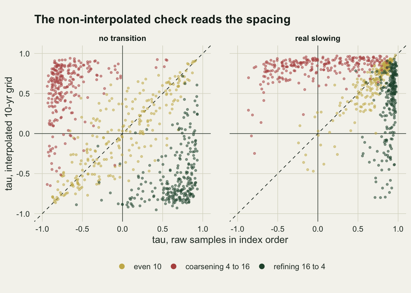
A null that goes through the same interpolation
The pipeline null works because it asks the right question: how large a tau this interpolation produces, at these ages, from a proxy with no change in memory. It needs the raw samples and their ages, one likelihood fit, and the interpolation step written as a function that can be applied to simulated values. Its false-alarm rate stayed near nominal in every null cell above, and its power on refining spacing is far above the standard test’s. It does not restore everything: on even spacing the two tests have similar power, and against coarsening spacing the pipeline null gives up some power, because its surrogates share the grid’s manufactured rise and a real slowing has to clear it.
A cheaper fix is to interpolate onto the coarsest spacing instead of the mean, so that almost no two grid points sit in the same gap. The chunk below uses a 16-year grid for the strong designs at \(\phi = 0.90\), 150 records per cell.
set.seed(33050)
cg_null <- run_cell(150, phi_base, phi_base, 4, 16, 16)
cg_slow <- run_cell(150, phi_base, phi_top, 16, 4, 16)
cg_slow_even <- run_cell(150, phi_base, phi_top, 10, 10, 16)
ou_scale_med <- median(cells_null[["even 10"]]$ou_scale)
On the 16-year grid the standard test flags 0.087 of the null records with coarsening spacing (pipeline null 0.027), against 0.288 on the 10-year grid, a standard error of 0.023 on the first. The real slowing with refining spacing is detected in 0.227 of the records by the standard test, up from 0.128 on the 10-year grid but still below the 0.393 of the pipeline null on the same coarse grid; with even spacing the coarse grid detects it in 0.407. So the coarse grid removes most of the false alarm at this \(\phi\) and part of the masking, at the cost of discarding samples in the finely spaced stretches; a record whose spacing ranges more widely than 4 to 16 years has no single coarse grid that keeps each gap from holding several grid points.
The fitted Ornstein-Uhlenbeck time scale is worth reporting for its own sake. On the even null records its median is 9.2 years against a true 9.5; set against the grid step, it says which part of the \(\phi\) curve a record sits on before any test is run.
What to report
Plot the gap between neighbouring samples against age, next to the indicator, and report its trend over the window. Spacing that coarsened from 4 to 16 years made the standard test flag 0.610 of records without a transition when the proxy had almost no memory at the grid step and 0.288 when its ten-year autocorrelation was 0.35; a drift from 8 to 12 years gave 0.140 and 0.084.
Report the interpolation step and the grid, and state the proxy’s memory at that step, for example as the time scale of a continuous-time AR(1) fitted to the raw samples at their ages. The same spacing trend matters much more for a proxy that is nearly uncorrelated from one grid step to the next than for one that is persistent.
Test the indicator against a null that goes through the same pipeline: simulate at the real sample ages, interpolate the same way, compute the same rolling statistic. The standard surrogate fitted to the gridded series answers a question about a regularly sampled record, which a core is not.
Do not read agreement or disagreement with the indicator computed on the non-interpolated samples as a validation. That indicator carries the opposite spacing artefact: under coarsening spacing it vetoes false rises and part of the real ones, and under refining spacing it rises on its own and cannot bring back a warning the grid has flattened.
When the spacing refines toward the event, as compaction tends to make it toward the young end of a core, report a missing warning with the power loss in mind. A flat indicator on such a record is weak evidence against critical slowing down.
Honest limits
The proxy is an annual AR(1) process, and the pipeline null fits exactly that model in continuous time, so the repair is correctly specified here by construction. A real proxy has measurement noise, may be smoothed by bioturbation over several centimetres, and may have more than one time scale; the null model would then be wrong in ways this simulation does not measure. The fitted time scale is a first check, not a guarantee. Only linear interpolation was tried: binning and kernel-based regridding weight the samples differently, and their artefact was not measured. An indicator that avoids the grid altogether, such as an Ornstein-Uhlenbeck time scale fitted to the raw samples in each window, was not tried either.
The ages are known exactly. A real core adds the dating error that the age-depth post follows into influx; here that source is switched off so that the spacing effect is seen alone, and a real record carries both. The spacing trend is linear in time with independent jitter, and the real pattern of years per centimetre is lumpier.
The real slowing raises only the memory, with the variance held at one. A system approaching a fold usually raises both, so the variance indicator would carry more information than it does here, and its weak response in the null cells is not a statement about its behaviour before a real transition.
Only one indicator, one window (half the record), one grid (10 years, plus the 16-year check) and one record length were simulated, and the surrogate tests use 49 surrogates each. Other indicators built from the same gridded series, such as the return rate or the spectral ratio, rest on the same neighbouring grid points and should be affected, but that was not measured. Replication is 250 records per cell in the table and in the raw-sample test, 300 for the strong drift and 150 for the mild drift on the \(\phi\) curve, 150 on the 16-year grid, and at least 80 per cell in the closed-form check, so no rate carries a Monte Carlo standard error above 0.041.
References
Braun T, Fernandez CN, Eroglu D, Hartland A, Breitenbach SFM, Marwan N 2022 Physical Review E 105(2):024206 (10.1103/PhysRevE.105.024206)
Ben-Yami M, Skiba V, Bathiany S, Boers N 2023 Nature Communications 14:8344 (10.1038/s41467-023-44046-9)
Dakos V, Scheffer M, van Nes EH, Brovkin V, Petoukhov V, Held H 2008 Proceedings of the National Academy of Sciences 105(38):14308-14312 (10.1073/pnas.0802430105)
Dakos V, Carpenter SR, Brock WA, Ellison AM, Guttal V, Ives AR, Kefi S, Livina V, Seekell DA, van Nes EH, Scheffer M 2012 PLoS ONE 7(7):e41010 (10.1371/journal.pone.0041010)
Rehfeld K, Marwan N, Heitzig J, Kurths J 2011 Nonlinear Processes in Geophysics 18(3):389-404 (10.5194/npg-18-389-2011)