library(ggplot2)
library(patchwork)

te_paper  <- "#f5f4ee"
te_ink    <- "#16241d"
te_body   <- "#2c3a31"
te_forest <- "#275139"
te_rust   <- "#b5534e"
te_gold   <- "#c9b458"
te_line   <- "#dad9ca"

theme_datasheet <- function() {
  theme_minimal(base_size = 12) +
    theme(plot.background  = element_rect(fill = te_paper, colour = NA),
          panel.background = element_rect(fill = te_paper, colour = NA),
          panel.grid.major = element_line(colour = te_line, linewidth = 0.3),
          panel.grid.minor = element_blank(),
          text             = element_text(colour = te_body),
          plot.title       = element_text(colour = te_ink, face = "bold"),
          plot.subtitle    = element_text(colour = te_body),
          axis.text        = element_text(colour = te_body))
}Pollen rate of change and uneven sample spacing
R
palaeoecology
pollen
time series
simulation
ecology tutorial
Pollen rate of change on unevenly spaced cores peaks at short gaps. Simulated in R: pooled time bins find a large turnover, one level per bin mostly does not.
A lake core has been cut into one centimetre slices, and every slice has had three hundred pollen grains counted. The age-depth model says the sediment took about twenty years to lay down each centimetre on average, but not evenly: some stretches accumulated fast and give slices a decade apart, others slowly and give slices forty years apart. The next number to go on the diagram is the rate of change: a dissimilarity between each pair of neighbouring samples, divided by the years between them, plotted against age. The tallest spike is where the text says the vegetation changed fastest.
Rate-of-change curves have a long history in palynology. Jacobson and Grimm (1986) assessed the rate of palynological change through the Holocene at Billy’s Lake in Minnesota, Bennett and Humphry (1995) analysed late-glacial and Holocene rates of vegetational change at two British sites, and Mottl et al. (2021) revisited the method, released the R-Ratepol package, and tested it on simulated sequences with uneven sampling. Their abstract reports that a moving window of time bins detected peak points correctly more than five times as often as working with individual levels. Nothing here is a new finding. The post measures, on simulated cores whose turnover date is known, which part of the calculation does the damage and which part of binning does the repair.
Three posts on this site sit next to the question without answering it. Age-depth models and what they do to a proxy shows how dating error turns a constant accumulation rate into a fluctuating influx record, and its advice is to push the proxy through a chronology ensemble and report the spread of the quantity of interest, naming the rate of change among them; it never computes one. Here the ages are known exactly, so everything that goes wrong is caused by the spacing alone. Derivatives of a GAM trend dates change in one smooth series on an even yearly grid, where the slope of a fitted curve is a well defined object. A pollen core is thirty taxa of count data on an uneven time axis, and the rate of change is a distance between noisy neighbours rather than a derivative. Weighted averaging transfer functions uses the squared chord distance for one job, finding the nearest modern analogue; this post uses its square root between successive samples.
A core with a turnover in the middle
Each simulated core has 120 slices. The years per centimetre follow a persistent random walk on the log scale, an autoregressive process with lag one correlation 0.8, rescaled to a mean of twenty years, so fast and slow stretches last for several slices. At a date drawn at random from the middle fifth of the core’s time span the pollen assemblage changes from one composition to another along a linear ramp lasting 150 years. The date is set from the age range of the core, not from a slice number, so it is unrelated to whether the local spacing is tight or loose, and because it is drawn afresh for every core it does not sit at the same place relative to the time bins used later. Counts are multinomial draws from the true proportions, and the dissimilarity is the chord distance: the Euclidean distance between square-root proportions, the square root of Overpeck’s squared chord distance. In vegan’s terms this is the Hellinger distance; R-Ratepol’s chord option calls vegan::vegdist(method = "chord") on proportions, which scales each row to unit length without taking square roots first, so the distance here is not the one that option computes.
n_taxa   <- 30       # pollen types
n_slice  <- 120      # one centimetre slices
yr_mean  <- 20       # mean years per centimetre
ar_phi   <- 0.8      # persistence of the log accumulation rate
acc_sd0  <- 0.35     # standard deviation of the log years per centimetre
dur0     <- 150      # turnover duration, years
bin_w    <- 100      # time bin width, years
tol_yr   <- 100      # a peak within this many years of the turnover centre is a hit
n_core   <- 400      # simulated cores per cell
grains   <- c(150, 300, 600, 2400)

rcomp <- function() { x <- rexp(n_taxa)^1.6; x / sum(x) }

make_core <- function(n_grain, dur = dur0, acc_sd = acc_sd0, change = TRUE,
                      shape = "linear", partial = FALSE, mix = 1) {
  z <- numeric(n_slice); z[1] <- rnorm(1, 0, acc_sd)
  innov <- rnorm(n_slice, 0, acc_sd * sqrt(1 - ar_phi^2))
  for (i in 2:n_slice) z[i] <- ar_phi * z[i - 1] + innov[i]
  yr_cm <- yr_mean * exp(z) / mean(exp(z))
  age <- cumsum(yr_cm) - yr_cm[1] / 2
  centre <- min(age) + diff(range(age)) * runif(1, 0.4, 0.6)   # not tied to the bin grid
  p_a <- rcomp(); p_b <- rcomp()
  if (partial) {                       # the two commonest taxa swap with the two rarest
    o <- order(p_a); p_b <- p_a
    p_b[o[n_taxa:(n_taxa - 1)]] <- p_a[o[1:2]]; p_b[o[1:2]] <- p_a[o[n_taxa:(n_taxa - 1)]]
  }
  p_b <- (1 - mix) * p_a + mix * p_b   # mix < 1 moves only part of the way to the second composition
  w <- if (!change) rep(0, n_slice) else if (shape == "linear") {
    pmin(pmax((age - (centre - dur / 2)) / dur, 0), 1)
  } else plogis((age - centre) / (dur / 6))
  probs <- outer(1 - w, p_a) + outer(w, p_b)
  counts <- t(apply(probs, 1, function(p) rmultinom(1, n_grain, p)))
  list(age = age, counts = counts, centre = centre, p_a = p_a, p_b = p_b)
}

chord_steps <- function(counts) {
  h <- sqrt(counts / rowSums(counts))
  sqrt(rowSums((h[-1, , drop = FALSE] - h[-nrow(h), , drop = FALSE])^2))
}
mids <- function(a) (a[-1] + a[-length(a)]) / 2
cv <- function(x) sd(x) / mean(x)
Six estimators are computed on every core, and each reports the age of its largest value. Two work on the original slices: the rate of change, chord distance divided by the age gap, and the chord distance left undivided. Four work on 100-year time bins, cut from the oldest sample upwards. A pooled bin sums the counts of all slices inside it and dates itself at their mean age. A selected bin keeps one slice picked at random, which is what the R-Ratepol documentation describes for its bins working units: one representative level from each time bin, chosen at random by default or as the level closest to the start of the bin. Each kind of bin is then used with and without the division by the age gap. R-Ratepol’s moving window repeats that selective binning with shifted bins, and its randomisation repeats the whole calculation; neither is reproduced here, so the binned arms below are this post’s own and should not be read as the package’s output.
peak_all <- function(core) {
  a <- core$age; cnt <- core$counts
  d_raw <- chord_steps(cnt); gap_raw <- diff(a)
  bin_id <- floor((a - min(a)) / bin_w)
  pooled <- rowsum(cnt, bin_id); age_pool <- as.vector(tapply(a, bin_id, mean))
  pick <- as.vector(tapply(seq_len(n_slice), bin_id,
                           function(ix) ix[sample.int(length(ix), 1)]))
  age_one <- a[pick]; d_one <- chord_steps(cnt[pick, , drop = FALSE])
  d_pool <- chord_steps(pooled)
  at_max <- function(m, v) m[which.max(v)]
  c(raw          = at_max(mids(a), d_raw / gap_raw),
    chord        = at_max(mids(a), d_raw),
    pooled_rate  = at_max(mids(age_pool), d_pool / diff(age_pool)),
    pooled_chord = at_max(mids(age_pool), d_pool),
    one_rate     = at_max(mids(age_one), d_one / diff(age_one)),
    one_chord    = at_max(mids(age_one), d_one),
    centre = core$centre, cor_inv = cor(d_raw / gap_raw, 1 / gap_raw),
    cv_raw = cv(gap_raw), cv_one = cv(diff(age_one)), cv_pool = cv(diff(age_pool)))
}
arm_names <- c("raw", "chord", "pooled_rate", "pooled_chord", "one_rate", "one_chord")
run_cell <- function(n, ...) do.call(rbind, lapply(seq_len(n), function(i) peak_all(make_core(...))))
hit_rate <- function(res, tol = tol_yr) colMeans(abs(res[, arm_names] - res[, "centre"]) <= tol)
One core first, at 300 grains per slice.
set.seed(4102)
ex <- make_core(300)
ex_gap <- diff(ex$age); ex_d <- chord_steps(ex$counts)
ex_df <- data.frame(age = mids(ex$age), gap = ex_gap, rate = ex_d / ex_gap, chord = ex_d)
ex_peak_rate <- ex_df$age[which.max(ex_df$rate)]
ex_peak_chord <- ex_df$age[which.max(ex_df$chord)]
ex_gap_at_peak <- ex_df$gap[which.max(ex_df$rate)]
ex_gap_rank <- rank(ex_df$gap, ties.method = "min")[which.max(ex_df$rate)]
ordinal <- function(k) if (k == 1) "smallest" else paste0(k, c("th", "st", "nd", "rd", rep("th", 6))[k %% 10 + 1], " smallest")
ex_turn_d <- sqrt(sum((sqrt(ex$p_a) - sqrt(ex$p_b))^2))
ex_floor <- median(ex_df$chord[abs(ex_df$age - ex$centre) > dur0])
ex_span <- range(ex_gap)
The spacing in this core runs from 8.0 to 39.1 years between neighbouring slices. The whole turnover moves the assemblage a chord distance of 0.95 from start to end, but spread over a 150-year ramp each twenty-year step carries only a fraction of that, while two neighbouring counts of the same composition already differ by a median of 0.229 from counting alone. The largest rate of change falls at 904 years, 146 years from the turnover centre at 1050, on a pair of slices 8.0 years apart, the smallest of the 119 gaps. The largest undivided chord distance falls at 1115 years.
ramp <- annotate("rect", xmin = ex$centre - dur0 / 2, xmax = ex$centre + dur0 / 2,
                 ymin = -Inf, ymax = Inf, fill = te_gold, alpha = 0.35)
p_gap <- ggplot(ex_df, aes(age, gap)) + ramp +
  geom_step(colour = te_body, linewidth = 0.5) +
  labs(x = NULL, y = "years between slices", title = "Spacing, rate and distance",
       subtitle = "shaded: the true turnover") + theme_datasheet()
p_rate <- ggplot(ex_df, aes(age, rate)) + ramp +
  geom_line(colour = te_rust, linewidth = 0.6) +
  geom_point(data = ex_df[which.max(ex_df$rate), ], colour = te_rust, size = 2.5) +
  labs(x = NULL, y = "chord / years") + theme_datasheet()
p_chord <- ggplot(ex_df, aes(age, chord)) + ramp +
  geom_line(colour = te_forest, linewidth = 0.6) +
  geom_point(data = ex_df[which.max(ex_df$chord), ], colour = te_forest, size = 2.5) +
  labs(x = "age (years from the top sample)", y = "chord distance") + theme_datasheet()
(p_gap / p_rate / p_chord) + plot_annotation(theme = theme_datasheet())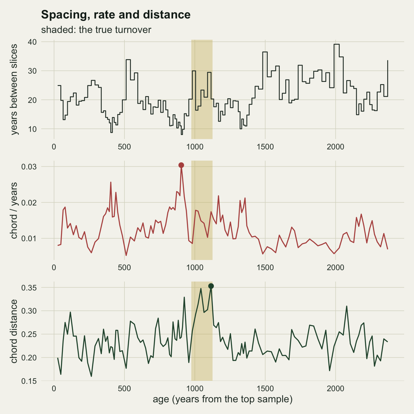
The division manufactures the peaks
A single core is an anecdote. The next chunk simulates 400 cores with a turnover and 400 cores with none at each of four pollen counts. On the cores with no change the largest value of any estimator is a peak that means nothing, and the share of those peaks that happen to land within 100 years of the date drawn for a turnover that never happened is the chance rate against which each hit rate has to be read.
set.seed(7361)
by_count <- lapply(grains, function(g) {
  list(turn = run_cell(n_core, g), flat = run_cell(n_core, g, change = FALSE))
})
hit_tab <- do.call(rbind, lapply(seq_along(grains), function(k) {
  data.frame(grains = grains[k], arm = arm_names,
             hit = hit_rate(by_count[[k]]$turn), chance = hit_rate(by_count[[k]]$flat))
}))
hit_tab$mcse <- sqrt(hit_tab$hit * (1 - hit_tab$hit) / n_core)
hv <- function(g, a, col = "hit") hit_tab[hit_tab$grains == g & hit_tab$arm == a, col]
cor_inv_med <- median(unlist(lapply(by_count, function(x) x$flat[, "cor_inv"])))
chance_raw <- range(hit_tab$chance[hit_tab$arm == "raw"])
chance_all <- range(hit_tab$chance)
mcse_max <- max(hit_tab$mcse)
On the cores with no change the rate of change is almost a picture of the spacing: its correlation with one over the gap, computed across the 119 neighbouring pairs of each core, has a median of 0.92. That part is arithmetic. When every neighbouring pair differs by about the same counting noise, dividing by the gap makes the shortest gaps the tallest spikes.
What matters is whether a real turnover can climb above that. At 150, 300 and 600 grains the largest rate of change lands within 100 years of the turnover in 10.0, 13.0 and 15.0 per cent of cores, against a chance rate between 8.0 and 12.5 per cent on cores with no turnover at all. At 2400 grains it reaches 40.5 per cent. The undivided chord distance, computed on the same counts, finds the turnover in 40.0, 65.5, 86.5 and 100.0 per cent. The pollen counts are the same in both columns; the only difference is the denominator. The largest Monte Carlo standard error of any hit rate in this section and the next is 2.5 percentage points.
div_tab <- hit_tab[hit_tab$arm %in% c("raw", "chord"), ]
div_tab$arm <- factor(div_tab$arm, levels = c("raw", "chord"),
                      labels = c("rate of change (chord / years)", "chord distance, undivided"))
ggplot(div_tab, aes(grains, hit, colour = arm)) +
  geom_errorbar(aes(ymin = hit - 2 * mcse, ymax = hit + 2 * mcse), width = 0.05, linewidth = 0.4) +
  geom_line(linewidth = 0.9) + geom_point(size = 2.2) +
  geom_point(aes(y = chance), shape = 21, fill = te_paper, size = 2.2, stroke = 0.8) +
  scale_x_log10(breaks = grains) +
  scale_colour_manual(values = c(te_rust, te_forest), name = NULL) +
  scale_y_continuous(limits = c(0, 1)) +
  labs(x = "pollen grains counted per slice (log scale)",
       y = "share of cores with the peak at the turnover",
       title = "Same counts, different denominator",
       subtitle = "open circles: chance on cores with no turnover") +
  theme_datasheet() + theme(legend.position = "bottom")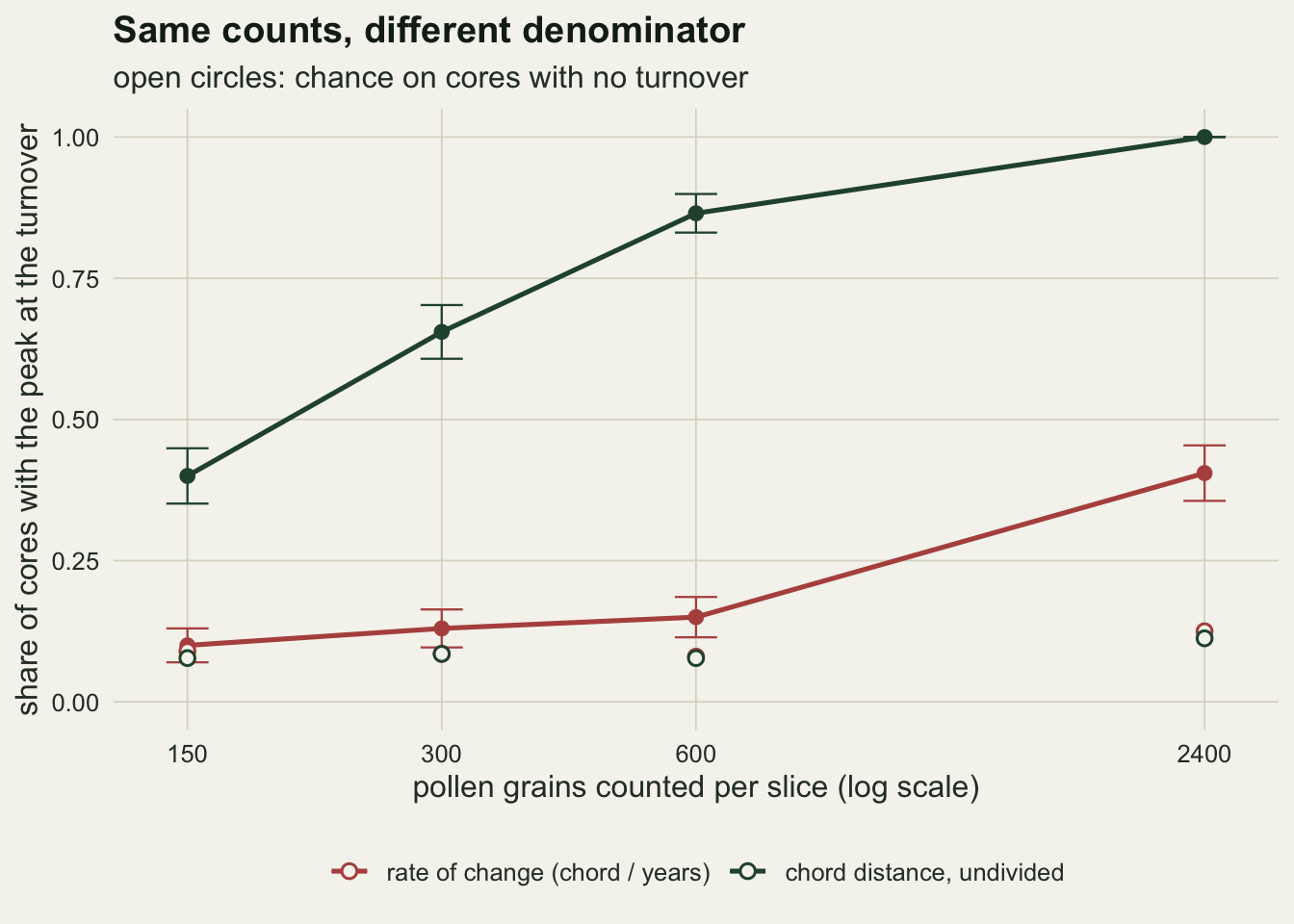
Which part of binning does the repair
Binning is the standard answer, and it changes three things at once. Each step between working units now spans about a hundred years instead of twenty, so a ramp moves the assemblage further per step while the counting noise per step stays where it was. Pooling adds the grains of several slices together. And the gap between working units changes character: bin means sit close to a hundred years apart, while two slices picked at random from adjacent bins can be almost touching or nearly two hundred years apart. The four binned arms pull these apart on the same cores.
cv_means <- colMeans(by_count[[2]]$turn[, c("cv_raw", "cv_one", "cv_pool")])
bin_tab <- hit_tab[hit_tab$arm %in% arm_names[3:6], ]
bin_tab$kind <- ifelse(grepl("pooled", bin_tab$arm), "pooled counts", "one slice per bin")
bin_tab$use <- ifelse(grepl("rate", bin_tab$arm), "divided by years", "undivided")
chance_bin <- range(hit_tab$chance[hit_tab$arm %in% arm_names[3:6]])
On a turnover that replaces the whole assemblage, pooled bins find it in every core at every count, whether or not the distance is divided by the years between bin means. Selected bins divided by their gap, the arm that follows R-Ratepol’s documented bins setting without the moving window, improve on the raw rate but stay well below the pooled bins until the largest count: 15.2, 23.2, 40.8 and 88.0 per cent from 150 to 2400 grains. Leave those same selected slices undivided and the hit rate is 98.0 per cent at 150 grains and 98.8 per cent at 600. The chance rates of the binned arms lie between 5.0 and 11.0 per cent.
So, on a turnover this large, the grains are not what separates the pooled bins from the selected ones. One slice per bin carries a fifth of the pooled count and still reaches 98.0 per cent at 150 grains once the division is removed. What separates them is the denominator. At 300 grains the coefficient of variation of the gap is 0.34 between neighbouring slices, 0.41 between the selected slices and 0.08 between pooled bin means. Selection makes the gaps less even than the original spacing, and dividing by them brings the manufactured peaks back; pooling makes the gaps nearly constant, and then dividing by them does no harm.
p_bin <- ggplot(bin_tab, aes(grains, hit, colour = kind, linetype = use)) +
  geom_line(linewidth = 0.9) + geom_point(size = 2) +
  scale_x_log10(breaks = grains) +
  scale_colour_manual(values = c(te_gold, te_forest), name = NULL) +
  scale_linetype_manual(values = c("solid", "22"), name = NULL) +
  scale_y_continuous(limits = c(0, 1)) +
  guides(colour = guide_legend(nrow = 2), linetype = guide_legend(nrow = 2)) +
  labs(x = "grains per slice (log scale)", y = "share of cores with the peak at the turnover",
       title = "Binned working units") +
  theme_datasheet() + theme(legend.position = "bottom")
unit_lab <- c("slices", "one slice\nper bin", "pooled\nbin means")
cv_df <- data.frame(unit = factor(unit_lab, levels = unit_lab),
                    cv = as.numeric(cv_means))
p_cv <- ggplot(cv_df, aes(unit, cv)) +
  geom_col(fill = c(te_rust, te_gold, te_forest), width = 0.6) +
  labs(x = NULL, y = "coefficient of variation of the gap",
       title = "Gap unevenness") +
  theme_datasheet()
(p_bin | p_cv) + plot_layout(widths = c(1.6, 1)) + plot_annotation(theme = theme_datasheet())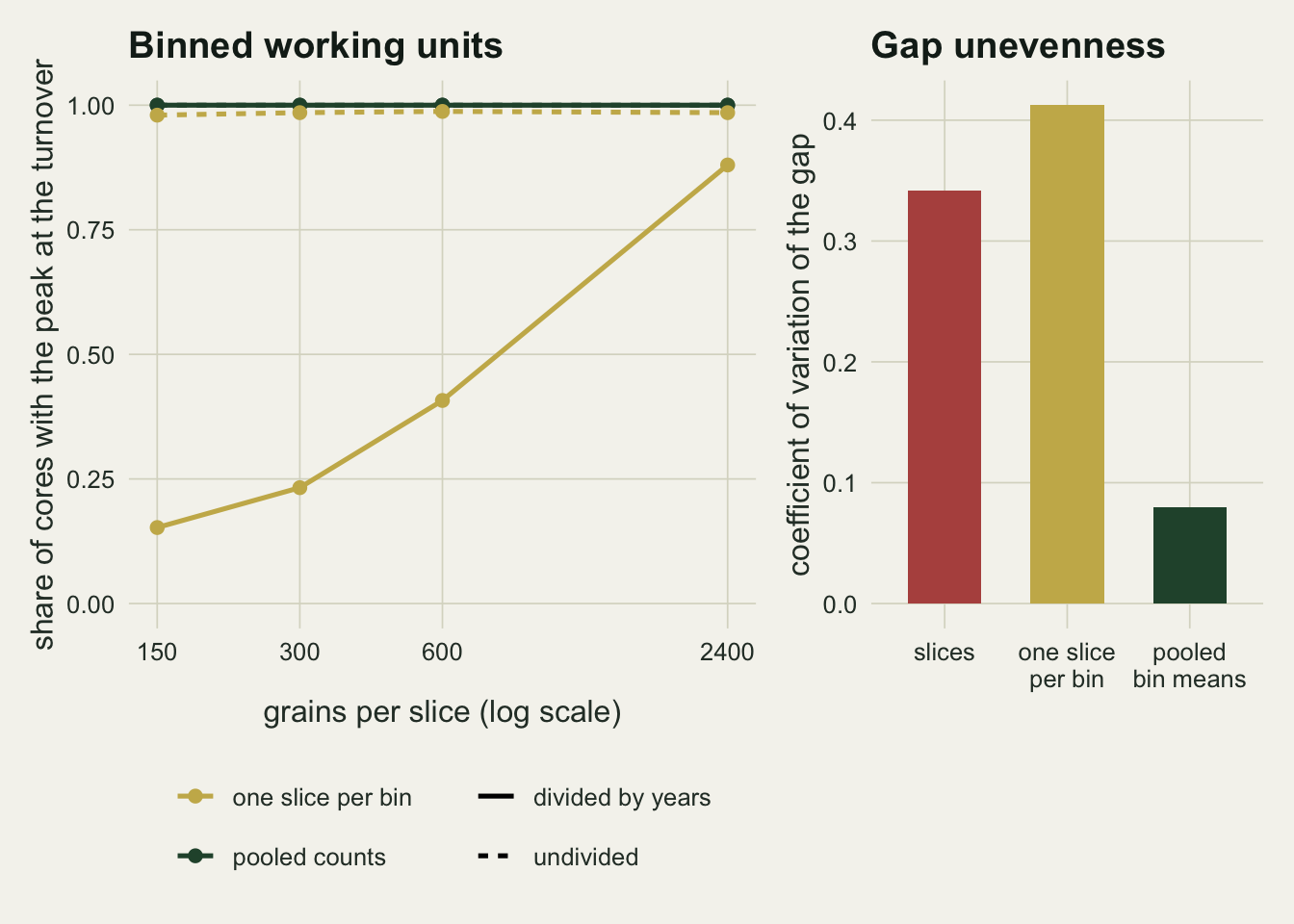
Slow turnovers and the score
A fixed hundred-year window around the centre is a fair score for a 150-year ramp. For a 400-year ramp the true rate of change is flat across the whole ramp, so a peak anywhere inside it is correct, and the narrow score would call most of those peaks misses. The next chunk counts both.
set.seed(2290)
dur_set <- c(50, 400)
by_dur <- lapply(dur_set, function(d) run_cell(n_core, 300, dur = d))
dur_hit <- function(k, tol = tol_yr) hit_rate(by_dur[[k]], tol)
pool_in_ramp_400 <- dur_hit(2, 400 / 2)["pooled_rate"]
chord_in_ramp_400 <- dur_hit(2, 400 / 2)["chord"]
raw_in_ramp_400 <- dur_hit(2, 400 / 2)["raw"]
w_even <- seq(0, 1, by = 0.05)             # a noiseless ramp in 20 equal steps
end_step <- replicate(n_core, {
  p_a <- rcomp(); p_b <- rcomp()
  d_step <- chord_steps(outer(1 - w_even, p_a) + outer(w_even, p_b))
  which.max(d_step) %in% c(1, length(d_step))
})
off400 <- abs(by_dur[[2]][, "pooled_rate"] - by_dur[[2]][, "centre"])
outer_share_400 <- mean(off400 > tol_yr & off400 <= 200) / mean(off400 <= 200)
med_off_pool_400 <- median(abs(by_dur[[2]][, "pooled_rate"] - by_dur[[2]][, "centre"]))
off_df <- do.call(rbind, list(
  data.frame(dur = "50-year turnover", off = by_dur[[1]][, "pooled_rate"] - by_dur[[1]][, "centre"], half = 25),
  data.frame(dur = "150-year turnover", off = by_count[[2]]$turn[, "pooled_rate"] - by_count[[2]]$turn[, "centre"], half = 75),
  data.frame(dur = "400-year turnover", off = by_dur[[2]][, "pooled_rate"] - by_dur[[2]][, "centre"], half = 200)))
off_df$dur <- factor(off_df$dur, levels = c("50-year turnover", "150-year turnover", "400-year turnover"))
At 300 grains a 50-year turnover is found within 100 years by the raw rate in 19.8 per cent of cores, by the undivided chord in 99.8, by pooled bins in 100.0 and by selected bins with division in 41.5. For the 400-year ramp the same four scores are 9.2, 18.8, 23.8 and 6.2 per cent, which read as though pooled bins lose the slow turnover. Score the same peaks by whether they fall inside the ramp and pooled bins place 97.2 per cent of them there, with a median distance of 130 years from the centre of a ramp whose half-width is 200. The undivided chord at slice level manages 41.2 per cent and the raw rate 17.2. The low narrow score for the slow turnover belongs to the score, not to the binning. Of the pooled peaks inside the 400-year ramp, 75.6 per cent sit in its outer half, more than 100 years from the centre. This part is arithmetic, not a simulation result. Along a linear ramp from composition a to composition b, the squared chord distance of a short step is proportional to the sum over taxa of (b - a)^2 / p, where p is the proportion at that point of the ramp; each term is convex in the mixing weight, so the sum is largest at one end or the other, and the largest step is the first or the last. On noiseless proportions stepped evenly through the ramp that held for all 400 random pairs of compositions (100.0 per cent). A slow turnover measured this way has its fastest steps at its edges, not its middle.
ggplot(off_df, aes(off)) +
  geom_rect(aes(xmin = -half, xmax = half, ymin = -Inf, ymax = Inf),
            data = unique(off_df[, c("dur", "half")]), inherit.aes = FALSE,
            fill = te_gold, alpha = 0.35) +
  geom_histogram(binwidth = 25, boundary = 0, fill = te_forest, colour = te_paper, linewidth = 0.2) +
  geom_vline(xintercept = c(-tol_yr, tol_yr), linetype = "dashed", colour = te_body, linewidth = 0.4) +
  facet_wrap(~ dur, ncol = 1) +
  coord_cartesian(xlim = c(-600, 600)) +
  labs(x = "peak age minus turnover centre (years)", y = "cores",
       title = "Pooled bins on slow and fast turnovers",
       subtitle = "shaded: the turnover; dashed: the 100-year score") +
  theme_datasheet() + theme(strip.text = element_text(colour = te_ink, face = "bold"))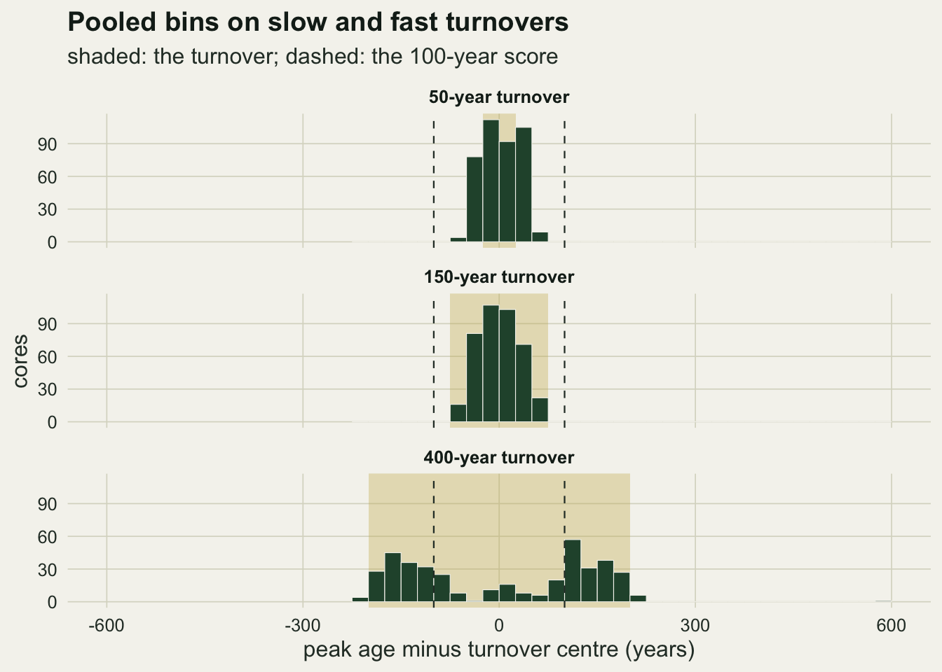
Checks on the design
The generating choices above could be carrying the result, so five of them were varied at 300 grains with everything else fixed: smoother and rougher accumulation, a logistic turnover in place of the linear ramp, a partial turnover in which only the two commonest taxa swap places with the two rarest while the other twenty-six keep their proportions, and a small turnover in which the assemblage moves only 15 per cent of the way from the first random composition towards the second.
set.seed(5518)
chk <- list(
  "accumulation sd 0.1" = run_cell(n_core, 300, acc_sd = 0.1),
  "accumulation sd 0.6" = run_cell(n_core, 300, acc_sd = 0.6),
  "logistic turnover"   = run_cell(n_core, 300, shape = "logistic"),
  "partial turnover"    = run_cell(n_core, 300, partial = TRUE),
  "small turnover"      = run_cell(n_core, 300, mix = 0.15))
turn_dist <- function(partial, mix = 1) {
  p_a <- rcomp(); p_b <- rcomp()
  if (partial) { o <- order(p_a); p_b <- p_a
    p_b[o[n_taxa:(n_taxa - 1)]] <- p_a[o[1:2]]; p_b[o[1:2]] <- p_a[o[n_taxa:(n_taxa - 1)]] }
  p_b <- (1 - mix) * p_a + mix * p_b
  sqrt(sum((sqrt(p_a) - sqrt(p_b))^2))
}
dist_full <- median(replicate(n_core, turn_dist(FALSE)))
dist_part <- median(replicate(n_core, turn_dist(TRUE)))
dist_small <- median(replicate(n_core, turn_dist(FALSE, mix = 0.15)))
cv_smooth <- colMeans(chk[["accumulation sd 0.1"]][, c("cv_raw", "cv_one")])
chk_tab <- rbind("design as above" = hit_rate(by_count[[2]]$turn), t(sapply(chk, hit_rate)))
big <- chk_tab[rownames(chk_tab) != "small turnover", ]
small <- chk_tab["small turnover", ]
chk_show <- data.frame(check = rownames(chk_tab),
                       rate = sprintf("%.1f", 100 * chk_tab[, "raw"]),
                       chord = sprintf("%.1f", 100 * chk_tab[, "chord"]),
                       pooled = sprintf("%.1f", 100 * chk_tab[, "pooled_rate"]),
                       selected = sprintf("%.1f", 100 * chk_tab[, "one_rate"]),
                       selected_undivided = sprintf("%.1f", 100 * chk_tab[, "one_chord"]))
knitr::kable(chk_show, row.names = FALSE,
col.names = c("check (300 grains)", "rate %", "chord %", "pooled bins %", "one per bin %", "one per bin, undivided %"))| check (300 grains) | rate % | chord % | pooled bins % | one per bin % | one per bin, undivided % |
|---|---|---|---|---|---|
| design as above | 13.0 | 65.5 | 100.0 | 23.2 | 98.5 |
| accumulation sd 0.1 | 33.8 | 57.5 | 100.0 | 27.3 | 98.8 |
| accumulation sd 0.6 | 9.0 | 72.5 | 100.0 | 28.0 | 98.5 |
| logistic turnover | 11.2 | 60.8 | 100.0 | 26.8 | 99.2 |
| partial turnover | 10.0 | 62.0 | 100.0 | 19.5 | 98.0 |
| small turnover | 5.8 | 14.5 | 51.0 | 8.5 | 31.0 |
Across the rows with a large turnover, pooled bins find it in every core and undivided selected slices in at least 98.0 per cent, while the selected bins divided by their gaps stay between 19.5 and 28.0 per cent. The raw rate is the arm that moves. Rougher accumulation, a log-scale standard deviation of 0.6, leaves it at 9.0 per cent, and smoother accumulation, 0.1, lifts it to 33.8 per cent, above the selected bins. With smooth accumulation the neighbouring slices have a gap coefficient of variation of 0.10, but the selected slices still have 0.40: random selection within bins creates uneven gaps even from nearly even spacing. The partial turnover is not a small change in chord terms, because the two commonest taxa carry a large share of the square-root proportions: its median chord distance from start to end is 0.81, against 0.87 for a full replacement by a second random composition.
The small turnover, with a median chord distance of 0.19 from start to end, is where the near-certainty goes. Pooled bins find it in 51.0 per cent of cores and undivided selected slices in 31.0 per cent; the undivided chord on slices manages 14.5, the selected bins with division 8.5 and the raw rate 5.8 per cent, against chance rates at 300 grains of 10.2, 10.2, 8.5, 8.5 and 8.5 per cent in the same order. The selected bins with division and the raw rate do no better than chance here, and the undivided chord on slices only a little better. The arms keep the order they had on the full turnover, but the near-certainty of pooled bins and undivided selected slices belongs to large turnovers.
What to report
Plot the years between samples under the rate-of-change curve. It costs one panel, and a reader who sees that the tallest spike sits over the shortest gap can judge it without any further analysis.
Say what the working units are. Levels, pooled bins and bins with one selected level are three different estimators, and on these cores with a full turnover they range from little above chance to near certainty on the same counts. For R-Ratepol, give the dissimilarity_coefficient, working_units, bin_size, bin_selection and number_of_shifts settings, and whether counts were rarefied.
If binning with one selected level per bin, check the spread of the gaps between the selected levels before dividing by them. Random selection makes those gaps more uneven than the original spacing (a coefficient of variation of 0.41 against 0.34 in the simulations here), and dividing by them left the selected-bin rate on the turnover in only 23.2 per cent of cores at 300 grains.
Report the undivided dissimilarity series alongside the rate. When the two agree on where the largest change is, the claim does not depend on the denominator; when they disagree, the rate’s peak needs a separate argument.
For slow changes, report the interval over which the rate is raised rather than the date of its maximum: on a chord scale the largest steps of a slow ramp sit near its start and end, so the maximum marks an edge of the change, not its middle.
Honest limits
The turnovers in the main design and in all but one check row move the assemblage a median chord distance of 0.81 or more from start to end, and the pooled and undivided selected arms reach near certainty on changes that large. The small-turnover row, with a median of 0.19 (22 per cent of the full replacement), brings pooled bins down to 51.0 per cent at 300 grains; no other magnitude, and no other count, was simulated for small changes.
The ages are known exactly. A real core has an estimated chronology, and the age-depth post measures how dating error on its own creates structure in derived rates; here that source is switched off so that the spacing effect can be seen alone, and a real core carries both.
R-Ratepol was not run. The selected-bin arm follows the package’s documented bins working units with random selection, but the moving window, which repeats the selection over shifted bins, the randomisation, which re-draws the selected level in every bin on each run and takes the median rate over runs, and the package’s peak-point detection were not reproduced. Averaging over shifts and runs spreads the selection, and it may recover part of what the single selection here loses; this post does not measure how much. Mottl et al. (2021) score detection of peak points by their own criteria, so the hit rates here are not comparable with the gain reported in their abstract.
The score is the position of the single largest value. A peak-detection rule that tests each value against a trend or a threshold would count differently, and a core with several real events would need a different score entirely. The chance rates on cores with no turnover are the only null used.
Counts are multinomial, with no extra variation between slices from taphonomy, differential preservation or counting error, so the noise floor here is a lower bound for a real core with the same count. Extra variation between slices raises that floor, which should make short gaps more damaging still; that was not simulated.
Every design has a single turnover near the middle of a 120-slice core with twenty years per centimetre on average. The 100-year bin is five mean spacings wide; bins much narrower than that leave fewer slices to pool and push the gaps between pooled means back towards the original spacing, which was not simulated.
References
Jacobson GL, Grimm EC 1986 Ecology 67(4):958-966 (10.2307/1939818)
Bennett KD, Humphry RW 1995 Review of Palaeobotany and Palynology 85(3-4):263-287 (10.1016/0034-6667(94)00132-4)
Mottl O, Grytnes JA, Seddon AWR, Steinbauer MJ, Bhatta KP, Felde VA, Flantua SGA, Birks HJB 2021 Review of Palaeobotany and Palynology 293:104483 (10.1016/j.revpalbo.2021.104483)