library(ggplot2)

te_paper  <- "#f5f4ee"
te_ink    <- "#16241d"
te_body   <- "#2c3a31"
te_forest <- "#275139"
te_rust   <- "#b5534e"
te_gold   <- "#c9b458"
te_line   <- "#dad9ca"

theme_datasheet <- function() {
  theme_minimal(base_size = 12) +
    theme(plot.background  = element_rect(fill = te_paper, colour = NA),
          panel.background = element_rect(fill = te_paper, colour = NA),
          panel.grid.major = element_line(colour = te_line, linewidth = 0.3),
          panel.grid.minor = element_blank(),
          text             = element_text(colour = te_body),
          plot.title       = element_text(colour = te_ink, face = "bold"),
          axis.text        = element_text(colour = te_body))
}

n_lake <- 80; n_sp <- 40; count_sum <- 400
ph_lo  <- 4.6; ph_hi <- 7.6

set.seed(31)
ph_true <- round(seq(ph_lo, ph_hi, length.out = n_lake) + rnorm(n_lake, 0, 0.05), 2)
sp_opt  <- runif(n_sp, ph_lo - 0.3, ph_hi + 0.3)
sp_tol  <- runif(n_sp, 0.35, 0.95)
sp_hgt  <- runif(n_sp, 20, 120)

# expected relative abundance of every species at a given pH
respond <- function(env) {
  outer(env, seq_len(n_sp),
        function(e, s) sp_hgt[s] * exp(-(e - sp_opt[s])^2 / (2 * sp_tol[s]^2)))
}
tally <- function(env, size = count_sum) {
  lam <- respond(env)
  t(apply(lam, 1, function(p) as.vector(rmultinom(1, size, p / sum(p)))))
}

calib  <- tally(ph_true)
pct <- calib / rowSums(calib)Weighted averaging transfer functions in R
R
palaeoecology
calibration
model diagnostics
ecology tutorial
Weighted averaging infers past pH from fossil assemblages, and it compresses the answer twice. Here is the deshrinking step and the analogue check it needs.
A transfer function turns a fossil assemblage into a number. Count the diatoms in a sediment slice, feed the percentages through a calibration built on modern lakes, and out comes the pH of that lake three hundred years ago, with a confidence band. The oldest and still the most widely used version of this is weighted averaging, and it is two lines of arithmetic: average the environment over the species, then average the species over the sample.
Both of those averages pull toward the middle. The estimate that comes out is a compressed version of the truth, systematically too high at the acid end and too low at the alkaline end, and the standard fix is a regression step called deshrinking that stretches it back out. That step is not cosmetic. It is a multiplier, it is fitted on the calibration set, and how large it is tells you something about the calibration set that a reported error statistic does not.
This post builds a calibration set with a known answer, runs weighted averaging by hand, measures the compression, and then reconstructs a synthetic core. It ends with the check that matters more than any of the arithmetic: whether the fossil assemblage has anything to do with the modern lakes at all.
Eighty lakes and forty species
Each species has a unimodal response to pH with its own optimum, tolerance and height. Counts are multinomial draws of a fixed count sum, which is how diatom and chironomid data are actually collected: a fixed number of valves or head capsules identified per slide.
show_sp <- order(sp_opt)[seq(1, n_sp, length.out = 12)]
grid_ph <- seq(ph_lo - 0.4, ph_hi + 0.4, length.out = 300)
curves  <- respond(grid_ph)
curves  <- curves / rowSums(curves)
d_curve <- do.call(rbind, lapply(show_sp, function(s)
  data.frame(ph = grid_ph, y = curves[, s], species = factor(s))))

ggplot(d_curve, aes(ph, y, group = species, colour = as.numeric(species))) +
  geom_line(linewidth = 0.8) +
  scale_colour_gradient(low = te_rust, high = te_forest, guide = "none") +
  labs(x = "pH", y = "expected relative abundance",
       title = "Twelve of the forty species") +
  theme_datasheet()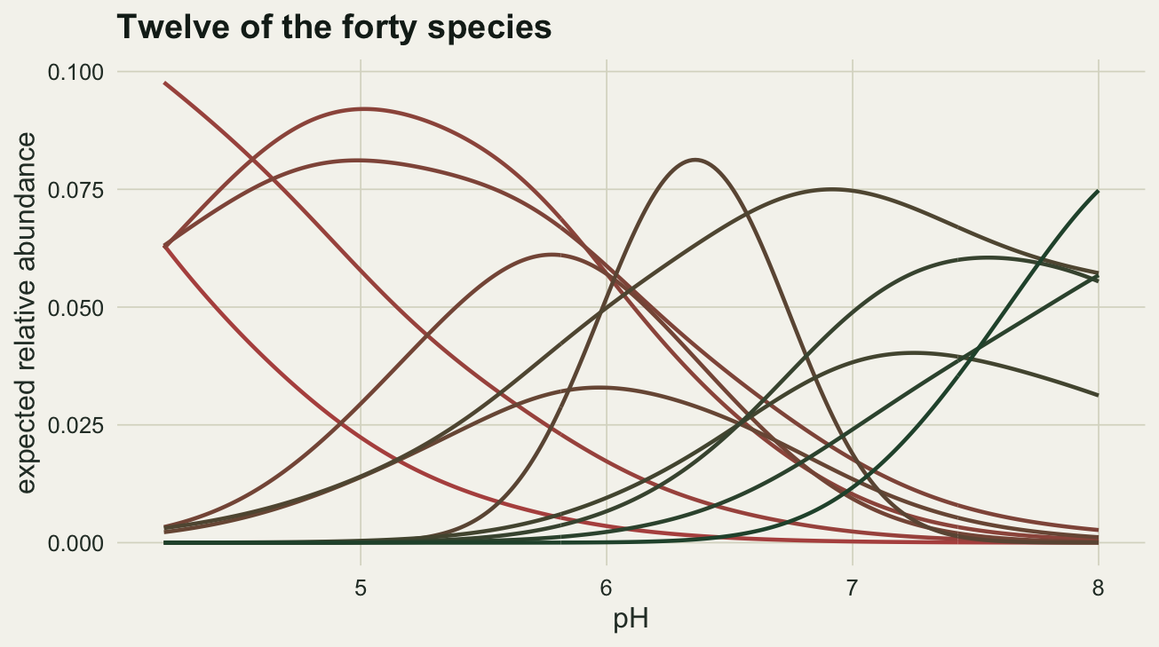
Two averages, and what they cost
The first average estimates each species optimum as the abundance weighted mean of the pH values where it was found. The second estimates each sample as the abundance weighted mean of the optima of the species in it.
wa_optima <- function(P, env) colSums(P * env) / colSums(P)
wa_sample <- function(P, optima) as.vector(P %*% optima / rowSums(P))

optima_hat <- wa_optima(pct, ph_true)
wa_raw     <- wa_sample(pct, optima_hat)

span_true <- diff(range(ph_true))
span_raw  <- diff(range(wa_raw))
shrunk    <- span_raw / span_true
The lakes span 3.04 pH units. The raw weighted averages span 1.57, which is 52 per cent of that. A species found only in the most acid lakes still gets an optimum pulled toward the centre, because the pH values it is averaged over are themselves a bounded sample; then each sample is an average over species whose optima have already been pulled in. The compression happens twice and it happens in the same direction both times.
inverse   <- lm(ph_true ~ wa_raw)
classical <- lm(wa_raw ~ ph_true)

pred_inv <- fitted(inverse)
pred_cls <- (wa_raw - coef(classical)[1]) / coef(classical)[2]

slope_inv <- unname(coef(inverse)[2])
slope_cls <- unname(1 / coef(classical)[2])
r_calib   <- cor(wa_raw, ph_true)
ratio_chk <- slope_inv / slope_cls

rmse <- function(a, b) sqrt(mean((a - b)^2))
rmse_raw <- rmse(wa_raw, ph_true)
rmse_inv <- rmse(pred_inv, ph_true)
rmse_cls <- rmse(pred_cls, ph_true)
span_inv <- diff(range(pred_inv)) / span_true
Deshrinking is the regression that undoes it, and it comes in two flavours that argue with each other in the literature. Inverse deshrinking regresses the known pH on the raw estimate and uses the fitted values. Classical deshrinking regresses the raw estimate on the known pH and then inverts the line. Their slopes here are 1.71 and 1.73. The ratio between the two is exactly the squared correlation of the calibration set: 0.9912 against an r squared of 0.9912. That identity is the whole argument. When a calibration set predicts itself well the two methods cannot differ, and when it does not, the difference between them is the least of the problems.
The prediction errors follow: 0.083 pH units for the inverse version and 0.083 for the classical one. Against the 0.374 of the undeshrunk estimate, the difference between the two flavours is not the interesting quantity. The interesting quantity is that skipping the step costs a factor of 4.5.
d_sh <- rbind(data.frame(truth = ph_true, est = wa_raw, kind = "raw weighted average"),
              data.frame(truth = ph_true, est = pred_inv, kind = "after deshrinking"))
d_sh$kind <- factor(d_sh$kind, levels = c("raw weighted average", "after deshrinking"))

ggplot(d_sh, aes(truth, est, colour = kind)) +
  geom_abline(slope = 1, intercept = 0, colour = te_ink, linetype = "dashed",
              linewidth = 0.6) +
  geom_point(size = 1.9, alpha = 0.85) +
  scale_colour_manual(values = c("raw weighted average" = te_rust,
                                 "after deshrinking" = te_forest), name = NULL) +
  labs(x = "known pH of the lake", y = "inferred pH",
       title = "Averaging twice pulls everything toward the middle") +
  theme_datasheet() +
  theme(legend.position = "bottom")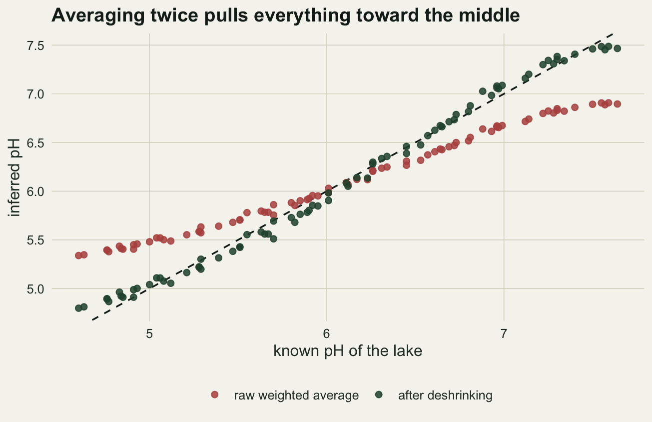
The slope is a noise multiplier
A deshrinking slope of 1.71 means the raw estimate is stretched by that factor, and so is everything else in it, including the part that is counting error rather than pH. How large the slope gets depends on how much of the gradient the calibration set covers.
gradient_run <- function(lo, hi, size, seed) {
  set.seed(seed)
  env <- round(seq(lo, hi, length.out = n_lake) + rnorm(n_lake, 0, 0.02 * (hi - lo)), 2)
  P   <- tally(env, size); P <- P / rowSums(P)
  est <- wa_sample(P, wa_optima(P, env))
  fit_i <- lm(env ~ est); fit_c <- lm(est ~ env)
  data.frame(gradient = hi - lo, counted = size,
             r = cor(est, env),
             slope_inverse = unname(coef(fit_i)[2]),
             slope_classical = unname(1 / coef(fit_c)[2]),
             rmse_inverse = rmse(fitted(fit_i), env),
             rmse_classical = rmse((est - coef(fit_c)[1]) / coef(fit_c)[2], env))
}
sweep_gr <- rbind(gradient_run(4.6, 7.6, count_sum, 31),
                  gradient_run(5.8, 6.8, count_sum, 31),
                  gradient_run(5.9, 6.5, count_sum, 31),
                  gradient_run(5.9, 6.5, 60, 31))
sweep_gr$rmse_pct <- 100 * sweep_gr$rmse_inverse / sweep_gr$gradient
print(transform(sweep_gr,
                r = round(r, 3),
                slope_inverse = round(slope_inverse, 2),
                slope_classical = round(slope_classical, 2),
                rmse_inverse = round(rmse_inverse, 3),
                rmse_classical = round(rmse_classical, 3),
                rmse_pct = round(rmse_pct, 1)), row.names = FALSE)
gradient counted r slope_inverse slope_classical rmse_inverse
3.0 400 0.996 1.72 1.73 0.075
1.0 400 0.992 6.46 6.56 0.036
0.6 400 0.979 15.97 16.66 0.036
0.6 60 0.895 12.93 16.16 0.079
rmse_classical rmse_pct
0.076 2.5
0.036 3.6
0.037 6.0
0.088 13.2On a fresh calibration set spanning 3.0 pH units the slope is 1.72. Over 0.6 units it is 16.0, because the raw estimates now occupy a sliver of an already short gradient. The error looks small in absolute terms, 0.036 pH units, and as a fraction of the gradient being reconstructed it has grown from 2.5 to 6.0 per cent.
The last row is the one where the choice of deshrinking finally shows up. Drop the count sum to 60 valves per sample on the short gradient and the calibration correlation falls to 0.89; the two slopes separate to 12.9 and 16.2, and the errors to 0.079 and 0.088. The textbook argument between the two methods is a real argument only in that corner: a weak calibration on a short gradient, which is also the corner where neither answer is worth much.
Reconstructing a core
A synthetic core, its pH rising smoothly through a sigmoid, run through the calibration built above.
n_slice  <- 30
core_ph  <- 5.0 + 3.2 / (1 + exp(-seq(-3, 3, length.out = n_slice)))
core_pct <- tally(core_ph); core_pct <- core_pct / rowSums(core_pct)

core_raw <- wa_sample(core_pct, optima_hat)
core_est <- unname(coef(inverse)[1] + coef(inverse)[2] * core_raw)

top_true <- max(core_ph); top_est <- max(core_est)
core_span_true <- diff(range(core_ph)); core_span_est <- diff(range(core_est))
The core runs from 5.15 to 8.05. The reconstruction recovers the shape. It does not recover the top: the core reaches 8.05 and the reconstruction stops at 7.60, having covered 87 per cent of the true change. The reason is not the arithmetic but the calibration set, whose most alkaline lake sits at 7.64. Weighted averaging is an average of optima estimated from those lakes, so it cannot return a value outside their range, and deshrinking rescales what is there rather than inventing an extrapolation. Every reconstruction that runs off the end of its calibration set flattens at the end, and the flattening looks exactly like a real plateau.
d_core <- rbind(data.frame(slice = seq_len(n_slice), ph = core_ph, kind = "true"),
                data.frame(slice = seq_len(n_slice), ph = core_est,
                           kind = "reconstructed"))

ggplot(d_core, aes(slice, ph, colour = kind)) +
  geom_hline(yintercept = max(ph_true), colour = te_gold, linewidth = 1) +
  annotate("text", x = 1, y = max(ph_true), label = "top of the calibration set",
           hjust = 0, vjust = -0.6, colour = te_gold, fontface = "bold", size = 3.3) +
  geom_line(linewidth = 1) +
  geom_point(size = 1.6) +
  scale_colour_manual(values = c(true = te_ink, reconstructed = te_forest),
                      name = NULL) +
  labs(x = "core slice, oldest at the left", y = "pH",
       title = "The reconstruction stops where the modern lakes stop") +
  theme_datasheet() +
  theme(legend.position = "bottom")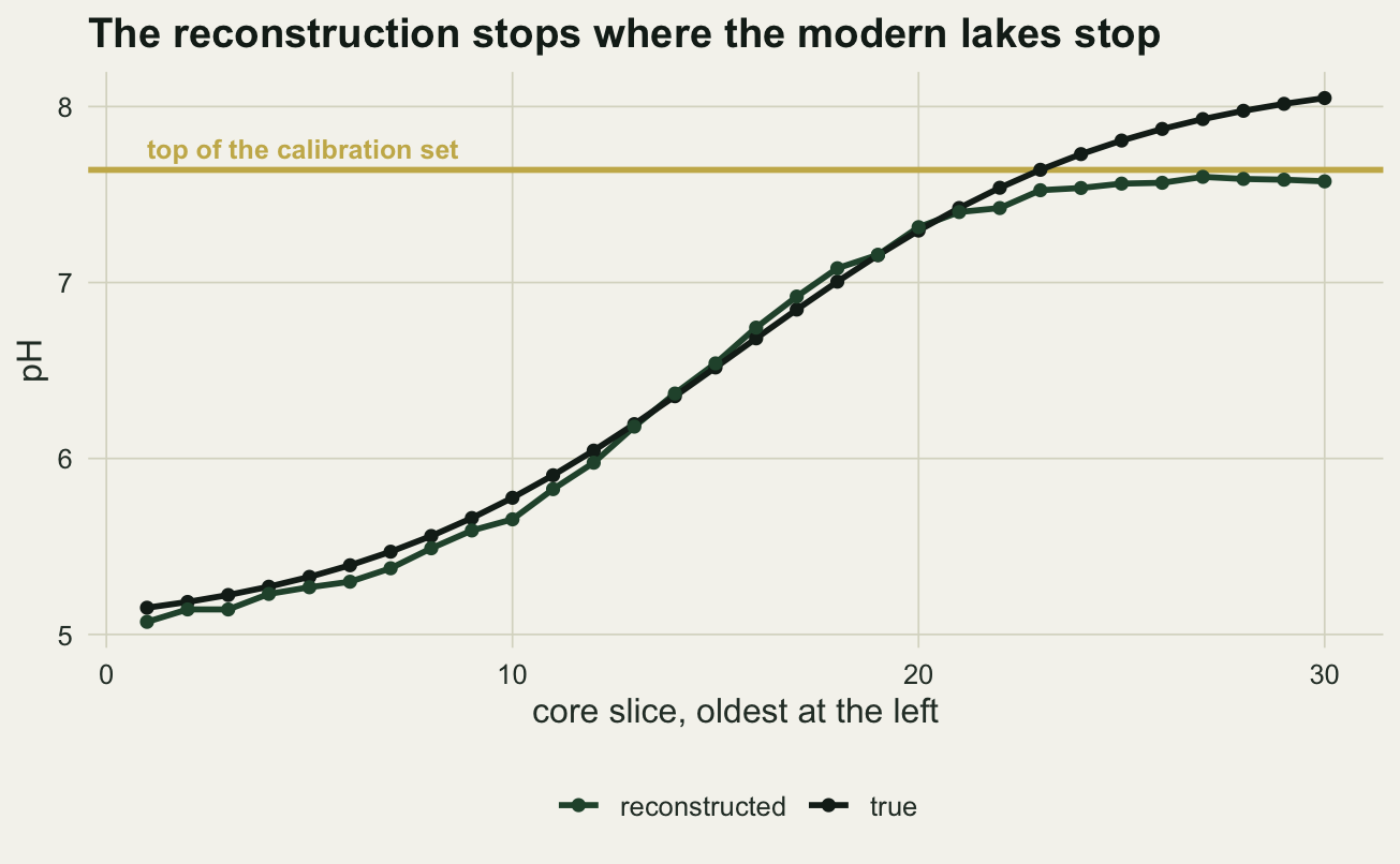
The check that matters: is there an analogue
Weighted averaging will return a number for any assemblage at all. It has no way of noticing that the fossil sample contains a combination of species that occurs in none of the modern lakes, because the arithmetic is an average over whatever species are present.
sq_chord <- function(a, B) apply(B, 1, function(b) sum((sqrt(a) - sqrt(b))^2))

# each calibration lake's distance to its own nearest neighbour, for a yardstick
nearest_calib <- sapply(seq_len(n_lake),
                        function(i) min(sq_chord(pct[i, ], pct[-i, , drop = FALSE])))

# an assemblage of strongly acid and strongly alkaline species together
odd <- rep(0, n_sp)
odd[order(sp_opt)[c(2, 3, n_sp - 2, n_sp - 1)]] <- c(0.30, 0.20, 0.25, 0.25)
odd_raw <- sum(odd * optima_hat) / sum(odd)
odd_est <- unname(coef(inverse)[1] + coef(inverse)[2] * odd_raw)
odd_dist <- min(sq_chord(odd, pct))
q_lev  <- 0.95
cut_95 <- unname(quantile(nearest_calib, q_lev))
That assemblage mixes species whose optima sit at opposite ends of the gradient, which no single lake in the calibration set does. Weighted averaging reports a pH of 5.99, comfortably mid gradient and indistinguishable from a real answer, with the same error bar as everything else.
The squared chord distance to the closest modern lake tells the other story: 1.24, against a 95th percentile of 0.052 for the distance between the calibration lakes and their own nearest neighbours. It is 24 times further from the modern data than a typical modern lake is from its nearest match. The check costs one function and it is the only part of this workflow that can say the reconstruction should not be attempted.
ggplot(data.frame(d = nearest_calib), aes(d)) +
  geom_histogram(bins = 26, fill = te_forest, colour = NA) +
  geom_vline(xintercept = odd_dist, colour = te_rust, linewidth = 1.1) +
  annotate("text", x = odd_dist, y = Inf, hjust = 1.05, vjust = 2,
           label = "the sample with no analogue", colour = te_rust,
           fontface = "bold", size = 3.5) +
  scale_x_log10() +
  labs(x = "squared chord distance to the nearest modern lake (log scale)",
       y = "calibration lakes",
       title = "How far the fossil sample sits from anything modern") +
  theme_datasheet()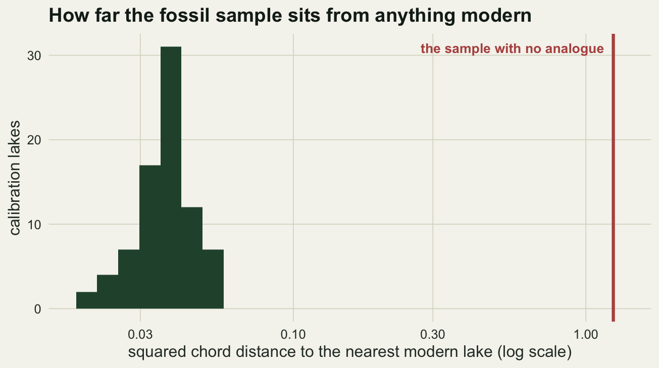
What to report
Report the deshrinking slope alongside the error statistic. It is one number, it is already fitted, and it says how much of the reconstruction is multiplication.
Report the range of the calibration set next to the range of the reconstruction. A reconstruction that touches either end of its calibration range is truncated there, and no error bar in the output will show it.
Report an analogue statistic for every fossil sample, not for the core as a whole. Cores usually have a few slices with no modern counterpart rather than a uniform problem, and those slices are often the interesting ones, because they are where the system was doing something it does not do now.
Report the cross validated error, and say how the folds were made. The apparent error of a calibration set fitted and evaluated on itself is an underestimate, and for spatially clustered lakes even a randomly folded cross validation is optimistic.
Honest limits
The species here have exactly Gaussian responses to one variable and nothing else. Real assemblages respond to several correlated variables at once, and a transfer function for pH built where pH covaries with total phosphorus will reconstruct some mixture of the two. Juggins set out this problem in 2013 in stronger terms than are used here, arguing that a good cross validated error is not evidence that the target variable is the one being tracked, and that the field’s standard diagnostics do not separate the two.
The compression measured here is a property of weighted averaging, not of transfer functions in general. Weighted averaging partial least squares, maximum likelihood Gaussian logit regression and the modern analogue technique each fail differently, and modern analogue in particular has no compression problem and a much worse extrapolation problem.
Tolerance downweighting, which divides each species contribution by its estimated tolerance, is left out. It usually helps a little and it makes the arithmetic longer without changing anything in this post.
The confidence intervals are left out too, and they deserve their own treatment. Bootstrapped sample specific errors for weighted averaging need the resampling to be done over the calibration lakes rather than the fossil counts, and the naive interval is far too narrow.
Finally, the squared chord threshold used above is the calibration set’s own nearest neighbour distribution, which is a defensible yardstick and not a standard one. Published cutoffs are usually taken from a percentile of the full modern dissimilarity distribution, which is a looser test, and there is no cutoff that makes a no-analogue reconstruction interpretable rather than merely flagged.
References
ter Braak CJF, van Dam H 1989 Hydrobiologia 178(3):209-223 (10.1007/BF00006028)
Birks HJB, ter Braak CJF, Line JM, Juggins S, Stevenson AC 1990 Philosophical Transactions of the Royal Society B 327(1240):263-278 (10.1098/rstb.1990.0062)
Juggins S 2013 Quaternary Science Reviews 64:20-32 (10.1016/j.quascirev.2012.12.014)