library(ggplot2)
library(patchwork)

te_paper  <- "#f5f4ee"
te_ink    <- "#16241d"
te_body   <- "#2c3a31"
te_forest <- "#275139"
te_rust   <- "#b5534e"
te_gold   <- "#c9b458"
te_line   <- "#dad9ca"

theme_datasheet <- function() {
  theme_minimal(base_size = 12) +
    theme(plot.background  = element_rect(fill = te_paper, colour = NA),
          panel.background = element_rect(fill = te_paper, colour = NA),
          panel.grid.major = element_line(colour = te_line, linewidth = 0.3),
          panel.grid.minor = element_blank(),
          text             = element_text(colour = te_body),
          plot.title       = element_text(colour = te_ink, face = "bold"),
          plot.subtitle    = element_text(colour = te_body),
          axis.text        = element_text(colour = te_body),
          strip.text       = element_text(colour = te_ink))
}Tuning proxy records manufactures synchrony
R
palaeoecology
time series
simulation
ecology tutorial
Shifting tie points within dating error makes independent proxy records correlate, and an effective sample size test often still passes them. Tested in R.
A lake core from a lowland basin and a peat core from an upland bog both carry a pollen record of the last ten thousand years, and both have been dated by radiocarbon at a handful of levels. The lake record shows a dip in tree pollen that the synthesis would like to call the same event as a dip in the peat record. The two chronologies put the dips a century and a half apart, which is inside the dating error of either core. So the second record is nudged: its dated levels are moved within their errors until the wiggles line up, and the aligned records go into a figure that shows two landscapes responding together.
The nudging is called tuning, and the problem with it is not that it is dishonest. Each shift is small and defensible, because every dated level really could sit anywhere inside its error. The problem is that the correlation between the two records is then used as evidence that they respond together, when the time axis of one record was chosen to make that correlation large. Blaauw set this out in 2012 under the title of a warning about aligning proxy archives, and an earlier study by Blaauw and colleagues compared Greenland and French records on chronologies that had not been tuned at all, so that the question of synchrony stayed open. This post is a demonstration of that known result, not a new one. What it adds is a set of numbers for one simple setting, and a measurement of whether the usual repair for autocorrelated series catches the problem.
That repair is the subject of two posts on this site. Temporal autocorrelation and effective sample size shows two independent persistent series looking correlated and corrects the test with an effective sample size, and the section on prewhitening in Checking a time series model makes the same point for the cross-correlation function. In both, the time axis is fixed and trusted. Here it is not: it has been fitted to the correlation, which is a different failure, and the question is whether a test built for the first one also covers the second. The chronology itself is the subject of Age-depth models and what they do to a proxy, which follows the error in one core into influx and into the date of a transition, but never puts a second record next to the first. Curve registration and functional PCA aligns seasons on their peaks, and that is legitimate there because every season has a real, well determined peak; two independent proxy records have no shared feature to register on, and a search for one will find one anyway.
The post measures what tuning does to the correlation between two records that share nothing, whether an effective sample size test sees through it, how the effect depends on the number of tie points and on the dating error, what an honest null for a tuned correlation looks like and how much power it leaves, and, briefly, what tuning does to a real lead of one record over the other.
Two records, each on its own clock
Both records are simulated on the same true time axis: a sample every 20 years over 10,000 years. Each is a first order autoregressive series with unit variance, the cheapest model of a proxy that carries one sample into the next. Record A is the reference and its chronology is taken as correct. Record B has its own age model: tie points every 2,000 years, each with a reported age that differs from its true age by a normal error with a standard deviation of 150 years, and linear interpolation between them, which is what a constant accumulation rate between dated levels gives. Where B’s chronology leaves the ends of the reference axis uncovered, those years are simply dropped from the comparison.
Tuning is a coordinate ascent. Each tie point in turn is moved to the offset, on a 20 year step within two standard deviations of its reported age, that gives the largest correlation between A and the resampled B, keeping the tie points in order; three passes over all tie points. That is a mechanical stand-in for moving tie points by eye until the wiggles agree, and a bound of two standard deviations is a generous reading of “within dating error”, not a bound taken from any published protocol. All of these design constants were fixed before any simulation ran.
dt_yr    <- 20
age_grid <- seq(0, 10000, by = dt_yr)
n_grid   <- length(age_grid)
sd_date  <- 150
phi_main <- 0.8
burn_len <- 300

ar1_series <- function(phi, n_out = n_grid) {
  e_in  <- rnorm(n_out + burn_len, sd = sqrt(1 - phi^2))
  x_out <- as.numeric(stats::filter(e_in, phi, method = "recursive"))
  x_out[(burn_len + 1):(burn_len + n_out)]
}

# weight of each tie point's age error at every point of the grid
hat_weights <- function(tie_age) {
  vapply(seq_along(tie_age), function(k) {
    unit_k <- as.numeric(seq_along(tie_age) == k)
    approx(tie_age, unit_k, age_grid)$y
  }, numeric(n_grid))
}

# B was sampled at the true ages; its chronology places each sample at est_age;
# read B back onto the reference grid (NA where the chronology does not reach)
resample_b <- function(b_val, est_age) {
  i_lo <- findInterval(age_grid, est_age)
  ok   <- i_lo > 0 & i_lo < n_grid
  out  <- rep(NA_real_, n_grid)
  i_ok <- i_lo[ok]
  frac <- (age_grid[ok] - est_age[i_ok]) / (est_age[i_ok + 1] - est_age[i_ok])
  out[ok] <- b_val[i_ok] + frac * (b_val[i_ok + 1] - b_val[i_ok])
  out
}

match_r <- function(a_val, b_ref) {
  ok <- !is.na(b_ref)
  cor(a_val[ok], b_ref[ok])
}

tune_ties <- function(a_val, b_val, tie_age, tie_err, sd_age, w_hat,
                      step_yr = 20, n_sweep = 3) {
  cand  <- seq(-2 * sd_age, 2 * sd_age, by = step_yr)
  d_off <- rep(0, length(tie_age))
  est0  <- age_grid + drop(w_hat %*% tie_err)
  best  <- match_r(a_val, resample_b(b_val, est0))
  for (s in seq_len(n_sweep)) for (k in seq_along(tie_age)) {
    base_est <- est0 + drop(w_hat %*% d_off) - w_hat[, k] * d_off[k]
    rep_tie  <- tie_age + tie_err + d_off
    r_cand   <- rep(-Inf, length(cand))
    for (j in seq_along(cand)) {
      rep_tie[k] <- tie_age[k] + tie_err[k] + cand[j]
      if (any(diff(rep_tie) <= 0)) next
      r_cand[j] <- match_r(a_val,
                           resample_b(b_val, base_est + w_hat[, k] * cand[j]))
    }
    if (max(r_cand) > best) {
      best     <- max(r_cand)
      d_off[k] <- cand[which.max(r_cand)]
    }
  }
  list(d = d_off, r = best,
       b_ref = resample_b(b_val, est0 + drop(w_hat %*% d_off)))
}

tie_six <- seq(0, 10000, by = 2000)
w_six   <- hat_weights(tie_six)
n_tie <- length(tie_six)set.seed(3200)
a_one <- ar1_series(phi_main)
b_one <- ar1_series(phi_main)
err_one <- rnorm(n_tie, 0, sd_date)
b_one_un <- resample_b(b_one, age_grid + drop(w_six %*% err_one))
tuned_one <- tune_ties(a_one, b_one, tie_six, err_one, sd_date, w_six)
r_one_un <- match_r(a_one, b_one_un)
r_one_tu <- tuned_one$r
shift_one_max <- max(abs(tuned_one$d))The first pair drawn has an untuned correlation of 0.201, already a sizeable value for two unrelated records, because both wander slowly and a few long excursions happen to coincide. After tuning it is 0.371, and no tie point moved by more than 280 years, inside the window of 300 years either way. Nothing about the records changed; only the clock of B did.
run_mean <- function(x) as.numeric(stats::filter(x, rep(1 / 11, 11), sides = 2))
one_df <- rbind(
  data.frame(age = age_grid, value = run_mean(a_one), record = "A, reference",
             panel = "B on its reported chronology"),
  data.frame(age = age_grid, value = run_mean(b_one_un), record = "B",
             panel = "B on its reported chronology"),
  data.frame(age = age_grid, value = run_mean(a_one), record = "A, reference",
             panel = "B after tuning"),
  data.frame(age = age_grid, value = run_mean(tuned_one$b_ref), record = "B",
             panel = "B after tuning"))
one_df$panel <- factor(one_df$panel,
                       levels = c("B on its reported chronology", "B after tuning"))
lab_df <- data.frame(panel = factor(levels(one_df$panel), levels = levels(one_df$panel)),
                     lab = c(sprintf("r = %.2f", r_one_un), sprintf("r = %.2f", r_one_tu)))

ggplot(one_df, aes(age, value, colour = record)) +
  geom_vline(xintercept = tie_six, colour = te_line, linewidth = 0.6) +
  geom_line(linewidth = 0.6, na.rm = TRUE) +
  geom_text(data = lab_df, aes(x = 9800, y = 1.9, label = lab),
            inherit.aes = FALSE, hjust = 1, colour = te_ink, size = 4) +
  facet_wrap(~ panel, ncol = 1) +
  scale_colour_manual(values = c(te_forest, te_rust), name = NULL) +
  labs(x = "true age (years)", y = "proxy value (standardised)",
       title = "Same records, different clock",
       subtitle = "grey verticals: true ages of B's tie points") +
  theme_datasheet() +
  theme(legend.position = "bottom")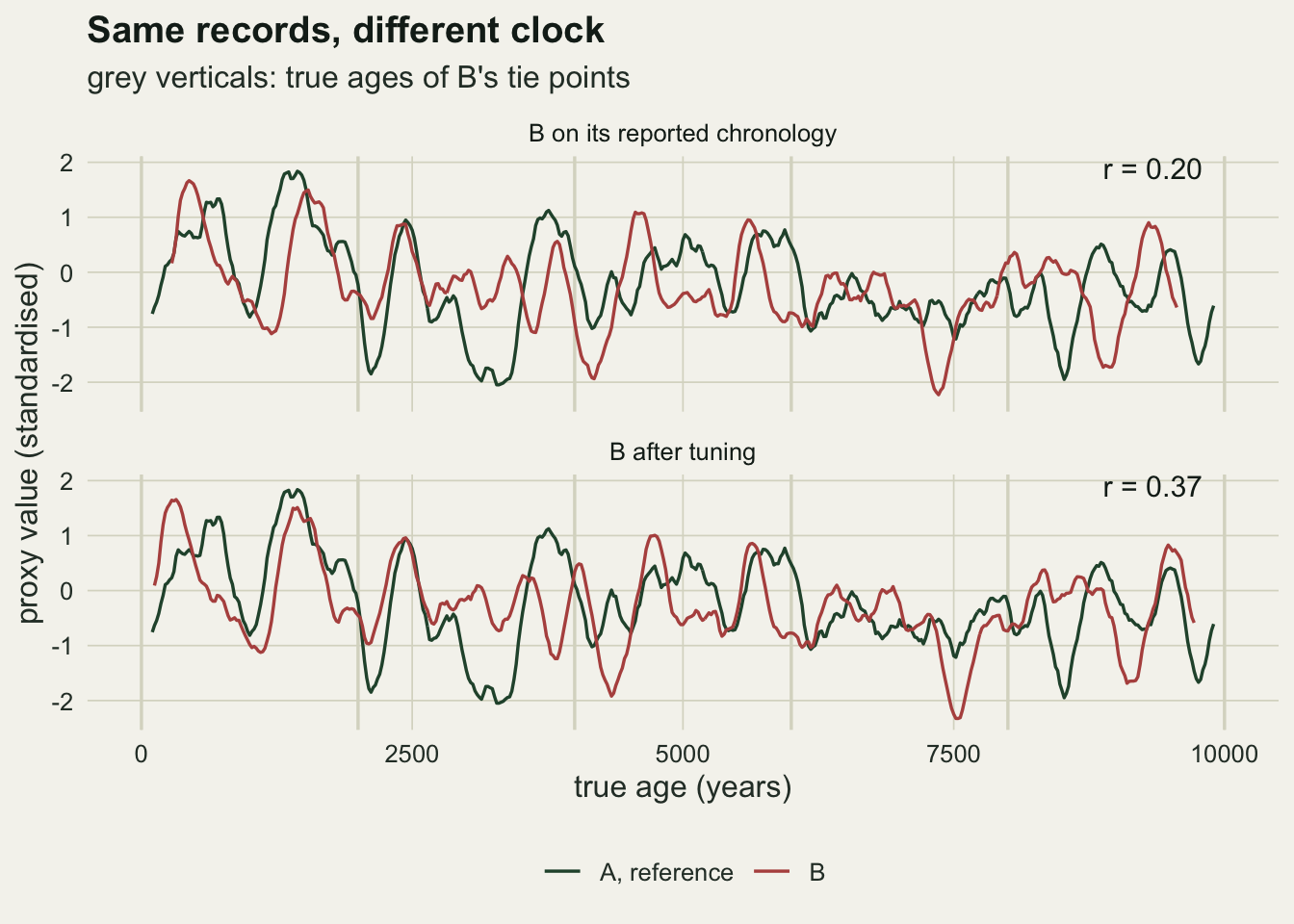
Tuning manufactures a correlation
lag1 <- function(x) {
  x <- x[!is.na(x)]
  cor(x[-1], x[-length(x)])
}
p_cor <- function(r_val, n_use) {
  t_val <- r_val * sqrt((n_use - 2) / (1 - r_val^2))
  2 * pt(-abs(t_val), n_use - 2)
}
# Bretherton et al. 1999: for two AR(1) series with lag one
# autocorrelations r1 and r2, n_eff = n (1 - r1 r2) / (1 + r1 r2)
n_eff_ar1 <- function(a_val, b_ref) {
  ok   <- !is.na(b_ref)
  r_ab <- lag1(a_val[ok]) * lag1(b_ref[ok])
  sum(ok) * (1 - r_ab) / (1 + r_ab)
}
lag_hat <- function(a_val, b_ref, max_step = 40) {
  steps <- -max_step:max_step
  r_lag <- vapply(steps, function(h) {
    if (h >= 0) {
      a_s <- a_val[1:(n_grid - h)]; b_s <- b_ref[(1 + h):n_grid]
    } else {
      a_s <- a_val[(1 - h):n_grid]; b_s <- b_ref[1:(n_grid + h)]
    }
    ok <- !is.na(b_s)
    cor(a_s[ok], b_s[ok])
  }, 0)
  steps[which.max(r_lag)] * dt_yr
}

run_pair <- function(phi, tie_age = tie_six, w_hat = w_six, sd_age = sd_date,
                     rho = 0, lag_yr = 0, n_ens = 0) {
  lag_n  <- lag_yr / dt_yr
  a_long <- ar1_series(phi, n_grid + lag_n)
  a_val  <- a_long[(lag_n + 1):(lag_n + n_grid)]
  b_val  <- rho * a_long[1:n_grid] + sqrt(1 - rho^2) * ar1_series(phi)
  tie_err <- rnorm(length(tie_age), 0, sd_age)
  b_un  <- resample_b(b_val, age_grid + drop(w_hat %*% tie_err))
  tuned <- tune_ties(a_val, b_val, tie_age, tie_err, sd_age, w_hat)
  r_un  <- match_r(a_val, b_un)
  out <- c(r_un = r_un, r_tu = tuned$r,
           p_naive_un = p_cor(r_un, sum(!is.na(b_un))),
           p_eff_un   = p_cor(r_un, n_eff_ar1(a_val, b_un)),
           p_naive_tu = p_cor(tuned$r, sum(!is.na(tuned$b_ref))),
           p_eff_tu   = p_cor(tuned$r, n_eff_ar1(a_val, tuned$b_ref)),
           n_eff_un   = n_eff_ar1(a_val, b_un),
           shift_mean = mean(abs(tuned$d)))
  if (lag_yr > 0) {
    out <- c(out, lag_un = lag_hat(a_val, b_un),
             lag_tu = lag_hat(a_val, tuned$b_ref))
  }
  if (n_ens > 0) {
    r_ens <- replicate(n_ens, match_r(a_val, resample_b(b_val,
      age_grid + drop(w_hat %*% (tie_err + rnorm(length(tie_age), 0, sd_age))))))
    out <- c(out, ens_hi = unname(quantile(r_ens, 0.975)))
  }
  out
}

n_main <- 300
n_high <- 150
set.seed(3201)
ind_80 <- replicate(n_main, run_pair(phi_main, n_ens = 100))
set.seed(3202)
ind_95 <- replicate(n_high, run_pair(0.95))

med_un_80 <- median(ind_80["r_un", ]); med_tu_80 <- median(ind_80["r_tu", ])
med_un_95 <- median(ind_95["r_un", ]); med_tu_95 <- median(ind_95["r_tu", ])
big_un_80 <- mean(abs(ind_80["r_un", ]) > 0.3)
big_tu_80 <- mean(ind_80["r_tu", ] > 0.3)
big_un_95 <- mean(abs(ind_95["r_un", ]) > 0.3)
big_tu_95 <- mean(ind_95["r_tu", ] > 0.3)
shift_med <- median(ind_80["shift_mean", ])
The single pair could be luck, so the same experiment was repeated on 300 independent pairs with a lag one autocorrelation of 0.80 and on 150 pairs with 0.95, a more persistent proxy. At 0.80 the median correlation is -0.006 on the reported chronology and 0.239 after tuning; at 0.95 the two medians are -0.020 and 0.196. A tuned correlation above 0.3 turned up in 22.3 per cent of pairs at the lower persistence and 25.3 per cent at the higher one, against 0.0 and 6.0 per cent of untuned correlations above 0.3 in absolute value.
The shifts that did this were modest. The median over pairs of the mean absolute shift per tie point was 177 years, a little over one standard deviation of the dating error, which is the kind of adjustment nobody reviewing the figure would question.
rdist_df <- rbind(
  data.frame(r = ind_80["r_un", ], chronology = "reported", phi = "lag one autocorrelation 0.8"),
  data.frame(r = ind_80["r_tu", ], chronology = "tuned", phi = "lag one autocorrelation 0.8"),
  data.frame(r = ind_95["r_un", ], chronology = "reported", phi = "lag one autocorrelation 0.95"),
  data.frame(r = ind_95["r_tu", ], chronology = "tuned", phi = "lag one autocorrelation 0.95"))

ggplot(rdist_df, aes(r, fill = chronology)) +
  geom_histogram(binwidth = 0.04, boundary = 0, position = "identity",
                 alpha = 0.7, colour = NA) +
  geom_vline(xintercept = 0, linetype = "dashed", colour = te_body, linewidth = 0.5) +
  facet_wrap(~ phi, ncol = 1, scales = "free_y") +
  scale_fill_manual(values = c(reported = te_forest, tuned = te_rust), name = NULL) +
  labs(x = "correlation between A and B", y = "record pairs",
       title = "Independent records, tuned into agreement",
       subtitle = "the two records share nothing in every pair") +
  theme_datasheet() +
  theme(legend.position = "bottom")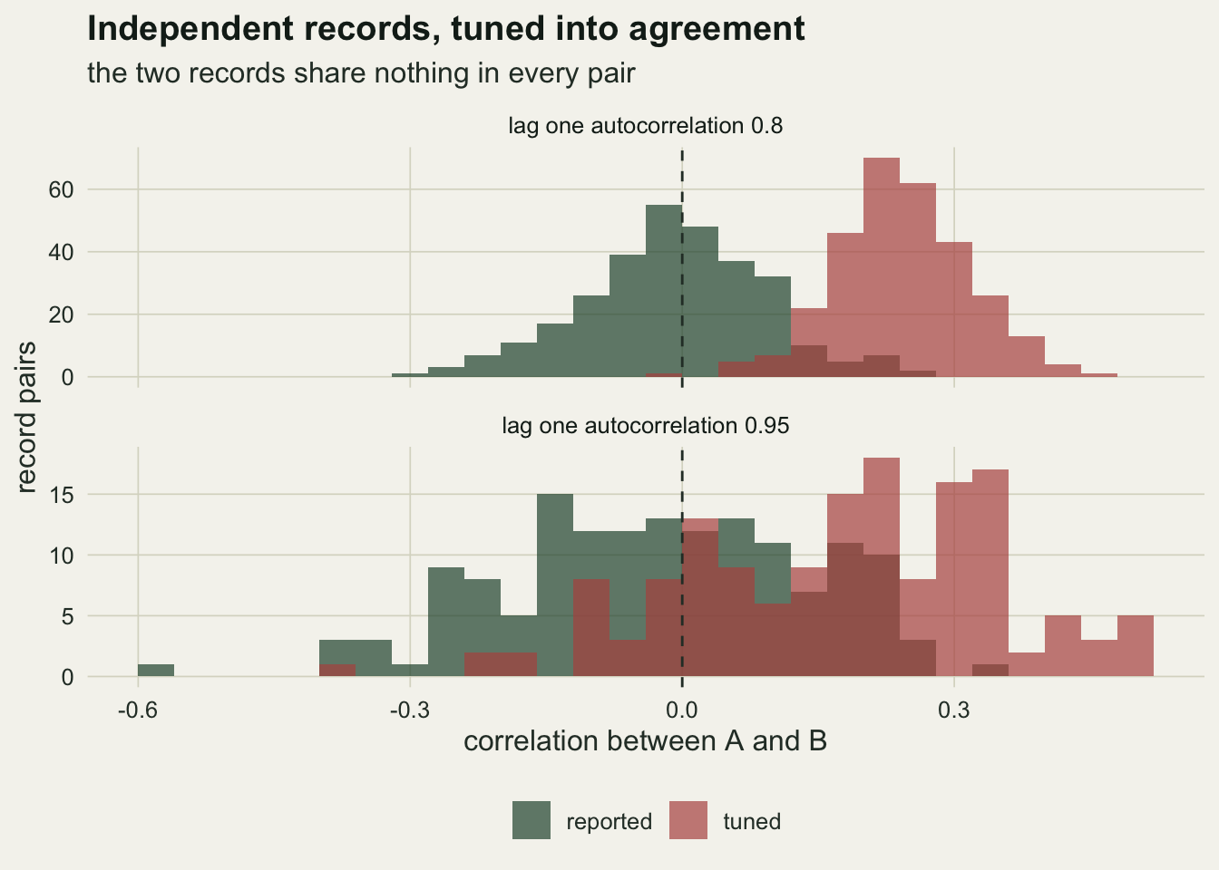
The effective sample size does not catch it
rej_tab <- function(m, lab) {
  p_rows <- c("p_naive_un", "p_eff_un", "p_naive_tu", "p_eff_tu")
  rate   <- rowMeans(m[p_rows, ] < 0.05)
  data.frame(test = rep(c("naive n", "effective n"), 2),
             chronology = rep(c("reported", "tuned"), each = 2),
             rate = unname(rate),
             se = sqrt(rate * (1 - rate) / ncol(m)),
             phi = lab)
}
fp_df <- rbind(rej_tab(ind_80, "lag one autocorrelation 0.8"),
               rej_tab(ind_95, "lag one autocorrelation 0.95"))
fp_get <- function(ph, te, ch) fp_df[fp_df$phi == ph & fp_df$test == te & fp_df$chronology == ch, ]
ph_lo <- "lag one autocorrelation 0.8"; ph_hi <- "lag one autocorrelation 0.95"
fp_eff_un_80 <- fp_get(ph_lo, "effective n", "reported"); fp_eff_tu_80 <- fp_get(ph_lo, "effective n", "tuned")
fp_nai_un_80 <- fp_get(ph_lo, "naive n", "reported"); fp_nai_tu_80 <- fp_get(ph_lo, "naive n", "tuned")
fp_eff_un_95 <- fp_get(ph_hi, "effective n", "reported"); fp_eff_tu_95 <- fp_get(ph_hi, "effective n", "tuned")
fp_nai_tu_95 <- fp_get(ph_hi, "naive n", "tuned")
neff_80 <- median(ind_80["n_eff_un", ]); neff_95 <- median(ind_95["n_eff_un", ])
n_theory_80 <- n_grid * (1 - phi_main^2) / (1 + phi_main^2)
crit_r_80 <- qt(0.975, neff_80 - 2) / sqrt(neff_80 - 2 + qt(0.975, neff_80 - 2)^2)
crit_r_95 <- qt(0.975, neff_95 - 2) / sqrt(neff_95 - 2 + qt(0.975, neff_95 - 2)^2)
The usual correction for two autocorrelated series replaces the number of samples with an effective number. For two first order autoregressive series with lag one autocorrelations r1 and r2, Bretherton and colleagues (their equation 31, a result that goes back to Bartlett) give the effective number as n (1 - r1 r2) / (1 + r1 r2), and the correlation is then tested with a t statistic on that many degrees of freedom. With both autocorrelations at 0.80 and the full grid this would be 110 samples; measured on the pairs, with lag one autocorrelations estimated from the records as they are compared, the median is 92.
On the reported chronology the correction does its job. At 0.80 a naive test rejects in 0.367 of independent pairs, and the effective sample size test in 0.060 (Monte Carlo standard error 0.014), which is near its nominal 0.05. On the tuned chronology the naive test rejects in 0.970 of pairs and the corrected one still in 0.700 (standard error 0.026). The correction repairs the autocorrelation problem it was built for but leaves most of the tuning problem in place, because a tuned correlation is the maximum of many correlations and the t distribution describes one.
The more persistent proxy does not follow the same pattern, so the result above does not carry over to every proxy. At 0.95 the median effective number is only 24, so a correlation needs to pass 0.40 to be called significant, against 0.20 at 0.80. The tuned correlations are similar in size (median 0.196), but the bar is about twice as high, and the corrected test rejects in 0.073 of tuned pairs (standard error 0.021), against 0.013 untuned. The naive test on the same tuned pairs rejects in 0.753. For a very smooth proxy the effective sample size is small enough that the correction swallows most of what tuning adds; for a moderately persistent one it does not. An analyst has no way to tell from a significant tuned correlation which of the two situations applies.
fp_df$test <- factor(fp_df$test, levels = c("naive n", "effective n"))
ggplot(fp_df, aes(test, rate, colour = chronology)) +
  geom_hline(yintercept = 0.05, linetype = "dashed", colour = te_body, linewidth = 0.5) +
  geom_errorbar(aes(ymin = rate - 2 * se, ymax = rate + 2 * se), width = 0.12,
                linewidth = 0.6, position = position_dodge(width = 0.4)) +
  geom_point(size = 2.8, position = position_dodge(width = 0.4)) +
  facet_wrap(~ phi) +
  scale_colour_manual(values = c(reported = te_forest, tuned = te_rust), name = NULL) +
  scale_y_continuous(limits = c(0, 1)) +
  labs(x = "correlation test", y = "false positive rate",
       title = "Correcting for autocorrelation is not correcting for tuning",
       subtitle = "dashed line: the nominal 5 per cent; bars: two standard errors") +
  theme_datasheet() +
  theme(legend.position = "bottom")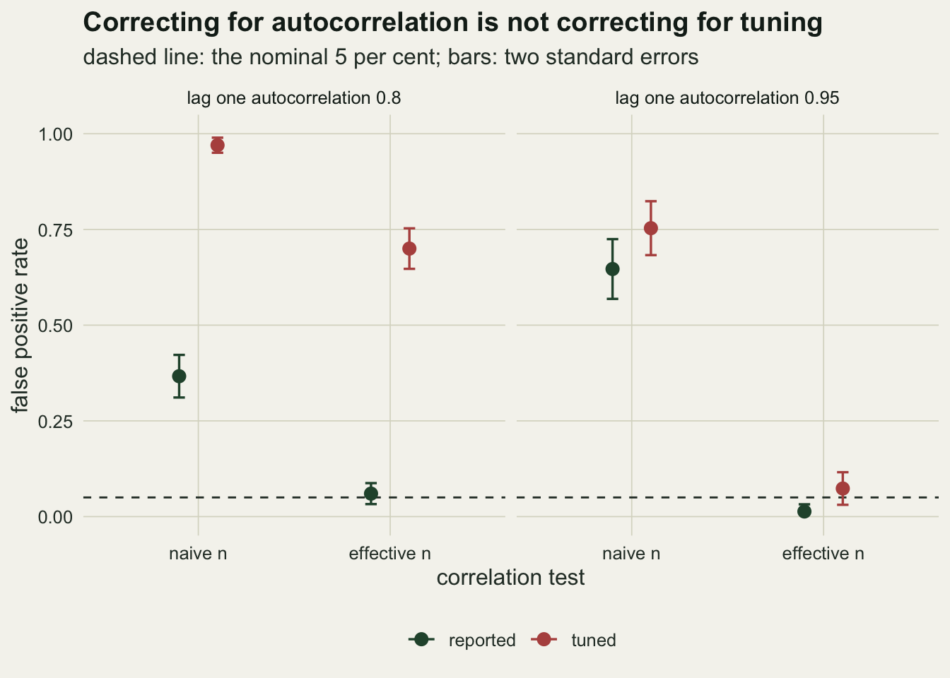
More tie points and wider errors give the search more room
tie_three  <- seq(0, 10000, by = 5000)
tie_twelve <- seq(0, 10000, length.out = 12)
n_cell <- 120
set.seed(3205)
k_three  <- replicate(n_cell, run_pair(phi_main, tie_three, hat_weights(tie_three)))
set.seed(3206)
k_twelve <- replicate(n_cell, run_pair(phi_main, tie_twelve, hat_weights(tie_twelve)))
set.seed(3207)
sd_fifty <- replicate(n_cell, run_pair(phi_main, sd_age = 50))
set.seed(3208)
sd_three <- replicate(n_cell, run_pair(phi_main, sd_age = 300))

cell_sum <- function(m, axis, level) {
  rate <- mean(m["p_eff_tu", ] < 0.05)
  data.frame(axis = axis, level = level, med_r = median(m["r_tu", ]),
             rate = rate, se = sqrt(rate * (1 - rate) / ncol(m)))
}
free_df <- rbind(
  cell_sum(k_three, "ties", 3),
  cell_sum(ind_80, "ties", 6),
  cell_sum(k_twelve, "ties", 12),
  cell_sum(sd_fifty, "sd", 50),
  cell_sum(ind_80, "sd", 150),
  cell_sum(sd_three, "sd", 300))
fr <- function(ax, lv) free_df[free_df$axis == ax & free_df$level == lv, ]
spacing_twelve <- diff(tie_twelve)[1]
The review question a palaeoecologist asks first is whether dating more levels helps. At a fixed dating error it makes things worse, because every tie point is another free parameter for the search. With 3 tie points the median tuned correlation is 0.179; with 6 it is 0.239; with 12, one every 909 years, it is 0.345. The effective sample size test calls the tuned pair significant in 0.358, 0.700 and 0.950 of independent pairs, each from 120 pairs except the middle one, which reuses the 300 pairs above.
The dating error sets the width of the window and acts the same way. With a standard deviation of 50 years the median tuned correlation is 0.148 and the corrected test rejects in 0.283 of pairs; with 300 years the median is 0.320 and the rejection rate 0.942. Even the tightest chronology here, with a window of a century either way, leaves the corrected test at several times its nominal level.
free_plot <- function(ax, x_lab) {
  sub_df <- free_df[free_df$axis == ax, ]
  sub_df$level <- factor(sub_df$level, levels = sub_df$level)
  ggplot(sub_df, aes(level, rate, group = 1)) +
    geom_hline(yintercept = 0.05, linetype = "dashed", colour = te_body, linewidth = 0.5) +
    geom_line(colour = te_rust, linewidth = 0.8) +
    geom_errorbar(aes(ymin = rate - 2 * se, ymax = pmin(1, rate + 2 * se)),
                  width = 0, colour = te_rust, linewidth = 0.6) +
    geom_point(colour = te_rust, size = 2.8) +
    geom_text(aes(y = rate - 0.07, label = sprintf("median r %.2f", med_r)),
              hjust = 0, nudge_x = 0.08, colour = te_ink, size = 3.3) +
    scale_x_discrete(expand = expansion(add = c(0.4, 1.2))) +
    scale_y_continuous(limits = c(0, 1.1), breaks = seq(0, 1, 0.25)) +
    labs(x = x_lab, y = "false positive rate") +
    theme_datasheet()
}
(free_plot("ties", "tie points (dating sd 150 years)") |
   free_plot("sd", "dating sd in years (6 tie points)")) +
  plot_annotation(title = "The more freedom the clock has, the more agreement it finds",
                  subtitle = "effective sample size test on tuned, independent records; dashed: 5 per cent",
                  theme = theme_datasheet())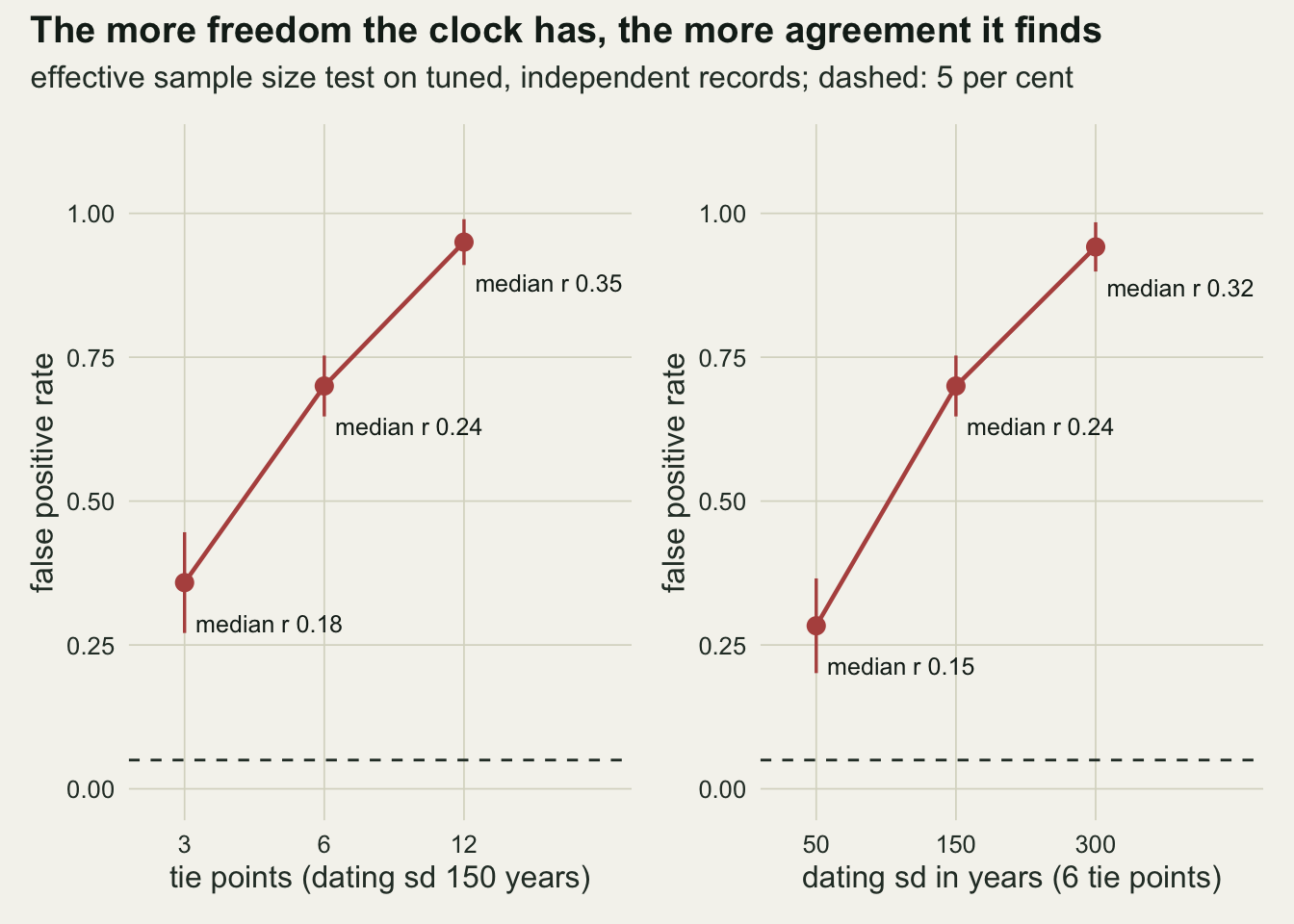
A null that is tuned the same way
ens_share_tu <- mean(ind_80["r_tu", ] > ind_80["ens_hi", ])
ens_share_un <- mean(ind_80["r_un", ] > ind_80["ens_hi", ])
n_null <- 200
set.seed(3203)
null_80 <- replicate(n_null, run_pair(phi_main))
r_crit  <- unname(quantile(null_80["r_tu", ], 0.95))
size_null <- mean(ind_80["r_tu", ] > r_crit)
size_null_se <- sqrt(size_null * (1 - size_null) / n_main)

rho_use <- 0.3
n_pow   <- 200
set.seed(3204)
cor_80 <- replicate(n_pow, run_pair(phi_main, rho = rho_use))
pow_null <- mean(cor_80["r_tu", ] > r_crit)
# one-sided tests at 5 per cent, the same size as the tuned null
pow_un   <- mean(cor_80["p_eff_un", ] < 0.10 & cor_80["r_un", ] > 0)
size_un  <- mean(ind_80["p_eff_un", ] < 0.10 & ind_80["r_un", ] > 0)
r_crit_un <- unname(quantile(null_80["r_un", ], 0.95))
size_un_null <- mean(ind_80["r_un", ] > r_crit_un)
pow_un_null  <- mean(cor_80["r_un", ] > r_crit_un)
pow_eff_tu <- mean(cor_80["p_eff_tu", ] < 0.05)
# the same 200 pairs are judged by both nulls, so the difference is paired
pow_diff_se <- sd((cor_80["r_tu", ] > r_crit) - (cor_80["r_un", ] > r_crit_un)) / sqrt(n_pow)
pow_se_max <- sqrt(0.25 / n_pow)
med_r_cor_un <- median(cor_80["r_un", ]); med_r_cor_tu <- median(cor_80["r_tu", ])
The honest reading of a tuned correlation starts from the chronology uncertainty the analyst already has. Drawing 100 alternative chronologies for each pair, by adding a fresh dating error to every reported tie age, gives a spread of correlations that the data are compatible with before anyone chooses among them. The tuned correlation exceeded the upper 2.5 per cent point of that ensemble in a share of 1.000 of the 300 independent pairs, and the untuned correlation in 0.003. The tuned value is not one of the chronologies the ensemble describes; it is the far edge of the whole family, found by search.
That points to the right null for a tuned correlation, which is the distribution of tuned correlations between records that are independent by construction and tuned by the same search. From 200 fresh independent pairs with the same persistence, tie points and window, the 95th percentile of the tuned correlation is 0.357. Applied to the 300 independent pairs of the earlier sections, which played no part in setting it, that critical value rejects in 0.060 of them (standard error 0.014).
Power needs a real relationship, and its strength was fixed before the run: B’s true values are 0.3 times A plus independent persistent noise, a modest shared signal. On the reported chronology the median correlation of those pairs is only 0.134, because dating error blurs the match. A fair comparison needs tests of the same size as the tuned null, which is one-sided at 5 per cent. The one-sided effective sample size test at 5 per cent finds a positive correlation in 0.370 of 200 pairs (it rejected in 0.040 of the independent pairs). An untuned simulated null, the 95th percentile of the untuned correlation over the same 200 null pairs, sits at 0.146, rejects in 0.060 of the independent pairs and finds the shared signal in 0.455. After tuning the median correlation is 0.366 and the tuned null rejects in 0.545 of pairs. The Monte Carlo standard error of each of these rates is at most 0.035. The effective sample size test on the tuned pairs rejects in 0.990, a number that means nothing, since it rejected in 0.700 of pairs with no relationship at all.
So tuning is not useless once it is tested properly. In this setting a tuned correlation judged against a tuned null had somewhat more power than an untuned correlation judged at the same size, by the effective sample size test or by an untuned simulated null; the margin over the untuned simulated null, 0.090, is 2.5 times its paired standard error (0.036, since the same 200 pairs are judged both ways), but each critical value is itself a percentile of only 200 null pairs, so the margin is suggestive rather than settled. The likely reason is that the search partly undoes the blurring that dating error causes to a real signal. The catch is the critical value: 0.357 is far above anything a t table would suggest, and it depends on the persistence, the number of tie points and the width of the window, all of which the analyst has to simulate for their own records.
A lead inside the window is absorbed by construction
n_lag <- 100
set.seed(3209)
lag_300 <- replicate(n_lag, run_pair(phi_main, rho = 0.9, lag_yr = 300))
set.seed(3210)
lag_600 <- replicate(n_lag, run_pair(phi_main, rho = 0.9, lag_yr = 600))
lag_sum <- function(m) c(un = median(m["lag_un", ]), tu = median(m["lag_tu", ]),
                         near_un = mean(abs(m["lag_un", ]) <= 100),
                         near_tu = mean(abs(m["lag_tu", ]) <= 100))
ls_300 <- lag_sum(lag_300); ls_600 <- lag_sum(lag_600)
The last question is what tuning does when B really does follow A, here by 300 years, with B’s true values 0.9 times A’s value from 300 years earlier plus independent noise. This part is close to a tautology and deserves one paragraph, not a figure. The search maximises the correlation at zero lag, and a lead of 300 years is inside the window of plus or minus 300 years, so the search removes it. Over 100 pairs the median lag estimated from the cross-correlation is 320 years on the reported chronology and 0 years after tuning, and 0.95 of tuned pairs put the lag within 100 years of zero against 0.03 untuned. A lead of twice the half-width behaves differently: for a 600 year lag the medians are 600 and 520 years, and only 0.16 of tuned pairs land within 100 years of zero, because a search that moves each tie point by at most 300 years cannot bring a 600 year offset to zero, and at zero lag the two records start out uncorrelated, so there is little for a local search to climb. Synchrony read off tuned records was put there by the objective whenever the true offset was inside the window.
What to report
State that a chronology was tuned, to what, and with how many tie points and what window. Those three numbers decide how much agreement the search could produce; in the cells above, the effective sample size test on independent tuned records rejected in anything from 0.283 to 0.950 of pairs, depending only on those settings.
Do not report a correlation between a record and the reference it was tuned to as evidence that the two respond together, and do not report its p-value, corrected or not. If a significance statement is needed, build the null by tuning independent surrogate records with the same persistence, tie points and window, as in the section above, and give the critical value alongside the observed correlation.
Report conclusions about synchrony or leads from untuned chronologies, with an ensemble of chronologies drawn from the dating errors, as Blaauw and colleagues did when comparing Greenland and France. A lead that sits within the tuning window is not recoverable from a tuned record: the 300 year lead above was put within 100 years of zero in 0.95 of tuned pairs.
Honest limits
The proxies are first order autoregressive series with a single persistence each, and both records share it. Real proxies have longer memory, trends and shared orbital scale structure, and a shared low frequency trend would make the untuned correlation positive before any tuning. How much tuning adds on top of a real trend was not measured.
The search is a coordinate ascent over a 20 year step with three passes. Someone matching wiggles by eye uses fewer, more deliberate moves on the features that stand out, may also stretch the depth scale between tie points, and may not confine themselves to two standard deviations. Whether a human search finds more or less agreement than this one is not something a simulation can settle; the direction of the effect does not depend on it.
The dating error is independent between tie points and normal, the accumulation rate between tie points is constant, and the reference record has no dating error of its own. Real age-depth models carry correlated errors between neighbouring dated levels, and a reference such as an ice core has its own chronology uncertainty. Both change the numbers.
The tuned null was built with the true persistence. An analyst would estimate it from the two records, and the critical value depends on it, as the difference between the two persistence levels shows; the null would then be approximate. Power was measured for one strength of shared signal, one persistence and one chronology design, from 200 pairs, so it is an example and not a power curve.
Correlations were computed only over the years B’s chronology covers, and that overlap changes a little with each tuning step. The search could therefore gain some correlation by trimming the ends. A check on fresh pairs puts that gain near zero.
n_trim <- 30
set.seed(3211)
trim_m <- replicate(n_trim, {
  a_val <- ar1_series(phi_main); b_val <- ar1_series(phi_main)
  t_err <- rnorm(n_tie, 0, sd_date)
  b_un  <- resample_b(b_val, age_grid + drop(w_six %*% t_err))
  tuned <- tune_ties(a_val, b_val, tie_six, t_err, sd_date, w_six)
  both  <- !is.na(b_un) & !is.na(tuned$b_ref)
  c(n_un = sum(!is.na(b_un)), n_tu = sum(!is.na(tuned$b_ref)), r_tu = tuned$r,
    r_common = cor(a_val[both], tuned$b_ref[both]))
})
trim_med <- apply(trim_m, 1, median)
Over 30 fresh independent pairs the median overlap is 496 samples on the reported chronology and 490 after tuning, out of 501, and the median tuned correlation is 0.255 on its own overlap against 0.259 on the years both chronologies cover.
References
Blaauw M 2012 Quaternary Science Reviews 36:38-49 (10.1016/j.quascirev.2010.11.012)
Blaauw M, Wohlfarth B, Christen JA, Ampel L, Veres D, Hughen KA, Preusser F, Svensson A 2010 Journal of Quaternary Science 25(3):387-394 (10.1002/jqs.1330)
Bretherton CS, Widmann M, Dymnikov VP, Wallace JM, Blade I 1999 Journal of Climate 12(7):1990-2009 (10.1175/1520-0442(1999)012<1990:TENOSD>2.0.CO;2)