library(ggplot2)
library(patchwork)

te_paper  <- "#f5f4ee"
te_ink    <- "#16241d"
te_body   <- "#2c3a31"
te_forest <- "#275139"
te_rust   <- "#b5534e"
te_gold   <- "#c9b458"
te_line   <- "#dad9ca"

theme_datasheet <- function() {
  theme_minimal(base_size = 12) +
    theme(plot.background  = element_rect(fill = te_paper, colour = NA),
          panel.background = element_rect(fill = te_paper, colour = NA),
          panel.grid.major = element_line(colour = te_line, linewidth = 0.3),
          panel.grid.minor = element_blank(),
          text             = element_text(colour = te_body),
          plot.title       = element_text(colour = te_ink, face = "bold"),
          plot.subtitle    = element_text(colour = te_body),
          axis.text        = element_text(colour = te_body))
}

a_gap <- 1.2; b_rec <- 0.9    # grazing into gap area, gap area into recruitment
g_ux  <- 0.9; g_uy  <- 1.1    # fertility into grazing, fertility into recruitment
n_plot <- 400; n_rep <- 500; ci_pct <- 95
eff_true <- a_gap * b_rec; direct_true <- 0L

sim_plots <- function(n, a = a_gap, b = b_rec, leak = 0) {
  fert  <- rnorm(n); graze <- g_ux * fert + rnorm(n)
  gap   <- a * graze + rnorm(n)
  seedl <- b * gap + leak * graze + g_uy * fert + rnorm(n)
  data.frame(graze = graze, gap = gap, seedl = seedl)
}Front-door adjustment when no instrument exists
R
causal inference
DAGs
mediation
ecology tutorial
Soil fertility confounds grazing and recruitment, and no instrument is available. A fully measured mechanism still identifies the total effect, in base R.
Four hundred permanent quadrats on a chalk grassland commons, one growing season. In each quadrat the survey recorded a grazing intensity index from dung pellet counts, the area of the quadrat surface sitting in vegetation gaps as a percentage of its area, and the number of seedlings that established the following spring. The question the grazing agreement turns on is simple: raise grazing intensity by one unit of the index and how many extra seedlings per square metre appear.
The slope of recruitment on grazing answers a different question. Stock does not spread itself evenly over a commons. The deeper, moister, more productive soils carry more forage, so they carry more animals, and the same soils independently support more seedlings through seed rain and summer water. Soil fertility is a common cause of the treatment and the outcome, and nobody sampled it. That is the standing problem of confounding and backdoor adjustment: the recipe there closes the backdoor path by conditioning on the confounder, and it needs the confounder in the data frame. It is not there.
The usual alternative is an instrument, something that shifts stocking density without touching recruitment by any other route, as in instrumental variables and 2SLS. On a working commons with negotiated stocking rights there is no such thing. What the survey does have is the mechanism. Grazing plausibly reaches seedlings by one route: animals remove standing biomass and litter, gaps open in the sward, and gaps are where small-seeded species can germinate. If gap area carries the whole of the grazing effect, then Pearl’s front-door criterion identifies the total effect from two regressions the survey can already fit, with soil fertility never measured and never modelled (Pearl 1995).
Sensitivity to unmeasured confounding opens by listing this site’s covariate-based toolkit: adjustment, weighting, matching and doubly-robust estimation, every one of which needs the confounder measured. Several designs on this site get round that requirement, and each pays for it with a different piece of study structure. Two-stage least squares needs an instrument. Regression discontinuity needs a threshold rule that decides who is treated, so that parcels either side of the line are near enough comparable. Event-study difference-in-differences needs repeated measurements either side of an intervention, and in exchange tolerates any confounder that stays fixed over time. Front-door adjustment asks for none of that structure: no instrument, no cut-off, no pre-period, only a measured mechanism. That is the case for knowing it, because a cross-section of quadrats surveyed once gives the other three nothing to work with. What it asks instead is one untestable assumption in place of another. This post measures what it buys in a simulation study, prices the assumption it depends on, and shows that the failure mode is nothing like the weak-instrument failure mode.
The naive slope is precise and wrong
The generating process is written out so the truth is known. Grazing intensity, gap area and recruitment are all centred on their site means, so each value is a deviation. Fertility raises grazing intensity and raises recruitment directly. Grazing raises gap area by a, gap area raises recruitment by b, and there is no other route from grazing to recruitment.
The total causal effect of grazing on recruitment is a times b, which is 1.08 seedlings per square metre per unit of the grazing index, and the direct effect that bypasses gaps is 0.
fert_x <- 0.75; fert_y <- 1.3          # fertility offset, so it is not over gap area
node <- data.frame(x = c(0, 1.5, 3, fert_x), y = c(0, 0, 0, fert_y),
  lab = c("grazing\nintensity", "gap\narea", "seedling\nrecruitment",
          "soil fertility\n(unmeasured)"))

trim <- function(x1, y1, x2, y2, pad_a, pad_b) {   # shorten an edge at both ends
  len <- sqrt((x2 - x1)^2 + (y2 - y1)^2)
  data.frame(x = x1 + (x2 - x1) * pad_a / len, y = y1 + (y2 - y1) * pad_a / len,
             xend = x2 - (x2 - x1) * pad_b / len, yend = y2 - (y2 - y1) * pad_b / len)
}
solid_edge <- rbind(trim(0, 0, 1.5, 0, 0.42, 0.30), trim(1.5, 0, 3, 0, 0.30, 0.55))
dash_edge  <- rbind(trim(fert_x, fert_y, 0, 0, 0.42, 0.36),
                    trim(fert_x, fert_y, 3, 0, 0.42, 0.42))
arrow_head <- arrow(length = unit(0.017, "npc"), type = "closed")

ggplot(node, aes(x, y)) +
  geom_segment(data = solid_edge, aes(x, y, xend = xend, yend = yend),
               colour = te_forest, linewidth = 0.8, arrow = arrow_head) +
  geom_segment(data = dash_edge, aes(x, y, xend = xend, yend = yend), colour = te_rust,
               linewidth = 0.8, linetype = "dashed", arrow = arrow_head) +
  annotate("curve", x = 0.2, y = -0.22, xend = 2.8, yend = -0.22, curvature = 0.28,
           colour = te_gold, linewidth = 0.7, linetype = "dotted",
           arrow = arrow_head) +
  annotate("text", x = 1.5, y = -0.66, label = "direct effect: assumed absent",
           colour = te_gold, size = 3.6) +
  geom_text(aes(label = lab), colour = te_ink, size = 3.9, lineheight = 0.95) +
  scale_x_continuous(limits = c(-0.55, 3.55)) +
  scale_y_continuous(limits = c(-0.95, 1.65)) +
  labs(title = "One measured mechanism, one unmeasured common cause") +
  theme_datasheet() +
  theme(panel.grid.major = element_blank(), panel.grid.minor = element_blank(),
        axis.title = element_blank(), axis.text = element_blank())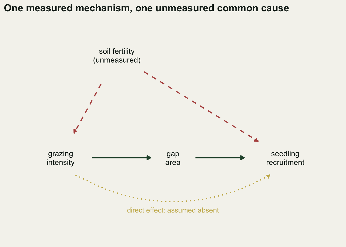
Fitting lm(seedl ~ graze) on 500 simulated surveys of 400 quadrats each shows what fertility costs.
three_est <- function(dat) {
  fit_a <- lm(gap ~ graze, data = dat); fit_b <- lm(seedl ~ gap + graze, data = dat)
  fit_n <- lm(seedl ~ graze, data = dat)
  a_hat <- coef(fit_a)[["graze"]]; b_hat <- coef(fit_b)[["gap"]]
  se_fd <- sqrt(b_hat^2 * summary(fit_a)$coefficients["graze", 2]^2 +
                a_hat^2 * summary(fit_b)$coefficients["gap", 2]^2)
  ci_n <- confint(fit_n)["graze", ]
  c(naive = coef(fit_n)[["graze"]], adjm = coef(fit_b)[["graze"]],
    fd = a_hat * b_hat, a_hat = a_hat, b_hat = b_hat,
    cov_n = as.numeric(ci_n[1] <= eff_true && eff_true <= ci_n[2]),
    cov_fd = as.numeric(abs(a_hat * b_hat - eff_true) <= 1.96 * se_fd))
}

set.seed(4021)
main_sim    <- replicate(n_rep, three_est(sim_plots(n_plot)))
main_mean   <- rowMeans(main_sim)
main_spread <- apply(main_sim, 1, sd)
naive_mean <- main_mean[["naive"]]
naive_bias <- naive_mean - eff_true
naive_cov  <- 100 * main_mean[["cov_n"]]
naive_pct  <- 100 * naive_bias / eff_true
The naive slope averages 1.624 against a truth of 1.08, so it overstates the grazing effect by 0.544 seedlings per square metre, or 50 per cent. Its replicate-to-replicate standard deviation is 0.062, and its 95 per cent confidence interval covers the true effect in 0 per cent of the 500 surveys. More quadrats would tighten that interval around the wrong number. This is the failure that the whole causal series exists to name, and in an ecological setting it is the normal case rather than the exception (Larsen, Meng and Kendall 2019).
Two regressions, multiplied, recover the total effect
The front-door formula asks for two things the survey has. First, the effect of grazing on gap area. Nothing confounds that pair: fertility does not reach gap area except through grazing, so lm(gap ~ graze) returns a cleanly. Second, the effect of gap area on recruitment, purged of fertility. Grazing is the only parent of gap area, so conditioning on grazing blocks the single backdoor path from gap area to recruitment, and lm(seedl ~ gap + graze) returns b on its gap coefficient. Multiply them.
In the linear Gaussian case the general front-door formula, which averages over the treatment distribution twice (Pearl 2009), collapses to that product. The estimator is three lines.
front_door <- function(dat) {
  a_hat <- coef(lm(gap ~ graze, data = dat))[["graze"]]
  b_hat <- coef(lm(seedl ~ gap + graze, data = dat))[["gap"]]
  a_hat * b_hat
}

fd_mean <- main_mean[["fd"]]; fd_bias <- fd_mean - eff_true
fd_cov  <- 100 * main_mean[["cov_fd"]]
a_mean  <- main_mean[["a_hat"]]; b_mean <- main_mean[["b_hat"]]
mc_se   <- main_spread[["fd"]] / sqrt(n_rep)
rep_mcse <- 100 * sqrt(0.01 * ci_pct * (1 - 0.01 * ci_pct) / n_rep)
adjm_mean <- main_mean[["adjm"]]
b_bias    <- b_mean - b_rec
Across the same 500 surveys the front-door estimate averages 1.0781, a bias of -0.0019 against a Monte Carlo standard error of 0.0039. The two ingredients land on their generating values: 1.1999 for the grazing-to-gap coefficient and 0.8985 for the gap-to-recruitment coefficient. The naive bias of 0.544 has gone, and what remains is smaller than the Monte Carlo noise of the study that measured it. The price is variance: the front-door standard deviation is 0.087 against 0.062 for the naive slope, because two estimated coefficients enter instead of one. Whether an interval built from that spread behaves as advertised is a separate question, and the next section measures it rather than assuming it.
est_long <- data.frame(est = c(main_sim["naive", ], main_sim["adjm", ], main_sim["fd", ]),
  which_est = rep(c("naive slope", "adjust for the mediator", "front-door"), each = n_rep))
est_long$which_est <- factor(est_long$which_est,
  levels = c("adjust for the mediator", "front-door", "naive slope"))

ggplot(est_long, aes(est, fill = which_est, colour = which_est)) +
  geom_density(alpha = 0.35, linewidth = 0.7) +
  geom_vline(xintercept = eff_true, linetype = "dashed", colour = te_ink,
             linewidth = 0.7) +
  annotate("text", x = eff_true, y = 0, label = "true total effect",
           colour = te_ink, size = 3.4, hjust = -0.06, vjust = -0.7) +
  scale_fill_manual(values = c(te_gold, te_forest, te_rust), name = NULL) +
  scale_colour_manual(values = c(te_gold, te_forest, te_rust), name = NULL) +
  labs(x = "estimated effect of grazing on recruitment", y = "density",
       title = "Only one of the three is aimed at the total effect",
       subtitle = sprintf("%d surveys of %d quadrats, fertility never measured",
                          n_rep, n_plot)) +
  theme_datasheet() + theme(legend.position = "bottom")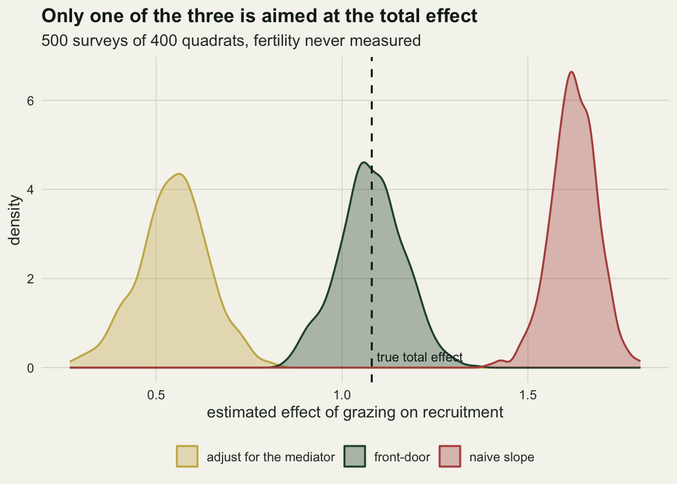
The interval holds here and fails in a regime this post is not in
The standard interval for a product of coefficients is the delta method, which is the standard error behind the Sobel test: square each coefficient, multiply it by the other coefficient’s squared standard error, add the two and take the root. Across the main study it covered the truth in 93.6 per cent of surveys. That reads as undercoverage and it is not evidence of any: 500 replicates locate a true coverage of 95 per cent only to within a Monte Carlo standard error of about 0.97 percentage points, so anything within two of those standard errors, between 93.1 and 96.9 per cent, is an ordinary draw from an interval that is working. Settling the question needs a longer run, and the answer turns out to depend on which regime is being asked about. The estimator and its delta standard error are written out in closed form below, which makes a long run cheap; the stopifnot line checks the closed form against the lm version before anything uses it.
fd_parts <- function(graze, gap, seedl) {
  n_obs <- length(graze)
  gz <- graze - mean(graze); gp <- gap - mean(gap); sy <- seedl - mean(seedl)
  s_zz <- sum(gz * gz); s_pp <- sum(gp * gp); s_pz <- sum(gp * gz)
  a_hat <- s_pz / s_zz; d_two <- s_pp * s_zz - s_pz^2
  se_a  <- sqrt(sum((gp - a_hat * gz)^2) / ((n_obs - 2) * s_zz))
  b_hat <- (s_zz * sum(gp * sy) - s_pz * sum(gz * sy)) / d_two
  z_hat <- (s_pp * sum(gz * sy) - s_pz * sum(gp * sy)) / d_two
  se_b  <- sqrt(sum((sy - b_hat * gp - z_hat * gz)^2) / (n_obs - 3) * s_zz / d_two)
  c(est = a_hat * b_hat, se = sqrt(b_hat^2 * se_a^2 + a_hat^2 * se_b^2),
    t_a = a_hat / se_a, t_b = b_hat / se_b)
}
fd_of <- function(dat) fd_parts(dat$graze, dat$gap, dat$seedl)

set.seed(2088); one_check <- sim_plots(n_plot)
stopifnot(all.equal(fd_of(one_check)[["est"]], front_door(one_check)))

n_cov <- 20000
regime <- data.frame(n = c(n_plot, n_plot, 50), a = c(a_gap, 0.1, 0.35),
                     b = c(b_rec, b_rec, 0.35))
set.seed(5108)
regime <- cbind(regime, t(vapply(seq_len(nrow(regime)), function(i) {
  reps <- replicate(n_cov, fd_of(sim_plots(regime$n[i], regime$a[i], regime$b[i])))
  hit  <- abs(reps["est", ] - regime$a[i] * regime$b[i]) <= 1.96 * reps["se", ]
  c(cover = 100 * mean(hit), mcse = 100 * sqrt(mean(hit) * (1 - mean(hit)) / n_cov),
    t_a = mean(reps["t_a", ]), t_b = mean(reps["t_b", ]),
    skew = mean((reps["est", ] - mean(reps["est", ]))^3) / sd(reps["est", ])^3)
}, numeric(5))))
At 20000 replicates the survey as simulated gives 94.57 per cent coverage with a Monte Carlo standard error of 0.16 points. That is a few tenths short of nominal, which is a real shortfall and a small one, and it is not skew: the sampling distribution of the product has a skewness of 0.058. The coefficients say why. The grazing-to-gap coefficient carries a t statistic averaging 32.3 and the gap-to-recruitment coefficient 13.9, and a product of two estimates that sharp is itself close to normal.
Weakening the mechanism on its own does not break it. Cutting the grazing-to-gap coefficient to 0.10 drops its t statistic to 2.7, and the interval still covers 95.25 per cent, because the second factor is untouched and the product stays close to linear in whichever factor is the noisy one. Both factors have to be imprecise at once. Row three sets the sample to 50 quadrats and both coefficients to 0.35, which is the shape of the simulation in mediation and bootstrapped indirect effects: t statistics of 3.3 and 1.9, skewness 0.61, and coverage down to 92.62 per cent. Same estimator, same delta formula, and the interval question bites there because both t statistics are small, not because the estimator is a product. Resampling is the usual answer in that regime and it is worth checking rather than assuming, so the comparison below is paired: each simulated survey gets both intervals.
n_bcov <- 1500; n_boot <- 299
w_n <- regime$n[3]; w_true <- regime$a[3] * regime$b[3]
set.seed(6613)
pair_hit <- replicate(n_bcov, {
  dat <- sim_plots(w_n, regime$a[3], regime$b[3])
  pt  <- fd_of(dat)
  bs  <- replicate(n_boot, { k <- sample.int(w_n, replace = TRUE)
    fd_parts(dat$graze[k], dat$gap[k], dat$seedl[k])[["est"]] })
  qq <- quantile(bs, c(0.025, 0.975))
  c(delta = as.numeric(abs(pt[["est"]] - w_true) <= 1.96 * pt[["se"]]),
    boot  = as.numeric(qq[[1]] <= w_true && w_true <= qq[[2]]))
})
pair_gain <- pair_hit["boot", ] - pair_hit["delta", ]
pair_diff <- 100 * mean(pair_gain); pair_se <- 100 * sd(pair_gain) / sqrt(n_bcov)
Over 1500 surveys in that regime the two coverage rates differ by -0.07 percentage points, percentile minus delta, against a standard error of 0.53 points on that paired difference. Resampling bought no measurable coverage there. The mediation post’s demonstration is about the shape of the interval rather than its coverage rate, and the skewness above says the shape really is wrong there; what the resampling did not do in this simulation is buy the missing coverage back. Neither interval is dependable when both paths are weak, which is a statement about sample size and effect size, not about the front-door criterion.
This is not adjusting for the mediator
The backdoor post is explicit that conditioning on a mediator is a mistake if the total effect is the target: it holds the intermediate fixed and reports only the leftover direct piece. This post puts a mediator in a regression on purpose. The two statements do not conflict, and the reason is visible in the coefficients rather than in the formula.
The fit lm(seedl ~ gap + graze) is used by both procedures, and they read different coefficients from it. The mediator adjustment reads the grazing coefficient, which averages 0.546 here. The true direct effect is 0, so that number is neither the total effect nor the direct effect: it is the direct effect plus whatever fertility leaves behind. The front-door estimate reads the gap coefficient from the same fit, which averages 0.8985 against a generating value of 0.9, off by -0.0015. One coefficient in that regression is identified and the other is not, and which is which follows from the graph: conditioning on grazing blocks the backdoor from gap area to recruitment, and nothing blocks the backdoor from grazing to recruitment.
The front-door formula is therefore not an adjustment set: it is a composition of two estimands, each identified by its own backdoor argument, and the product is the total effect rather than a residual direct effect. The mediator sits in the second regression as a response variable’s predictor whose own coefficient is wanted, not as a covariate whose presence is meant to clean up the grazing slope.
A sharper contrast with the mediation post, because it works on the same kind of mediator and reaches the opposite conclusion. Its closing caveat is that a confidence interval for the product excluding zero “does not establish that the mediator causes the response rather than the reverse, nor that no unmeasured variable drives both”. That is a warning that the mediated path is itself hostage to unmeasured confounding. Front-door adjustment turns the same product into an identification result, and the fee is paid up front: the arrow from grazing to recruitment must be absent, the arrows into and out of gap area must be as drawn, and gap area must be free of its own unmeasured confounding with recruitment. Nothing in the data checks any of that. The mediation post declines to make the causal claim; this post makes it, having bought it with assumptions.
The bias is the leak, one for one
Complete mediation is the assumption at risk. Livestock trample seedlings and disperse seed in dung, and neither of those routes passes through gap area. Add a direct grazing-to-recruitment edge of size leak and the true total effect becomes a times b plus leak, while the front-door estimand still targets the mediated path alone. The sweep below uses common random numbers: within a replicate, fertility, grazing, gap area and the recruitment noise are drawn once and only the direct edge is varied. That removes the sampling noise from the comparison and makes the pattern exact rather than approximate.
leak_set <- c(0, 0.1, 0.2, 0.4)
leak_one <- function(n) {
  fert  <- rnorm(n); graze <- g_ux * fert + rnorm(n)
  gap   <- a_gap * graze + rnorm(n); noise <- g_uy * fert + rnorm(n)
  a_hat <- coef(lm(gap ~ graze))[["graze"]]
  vapply(leak_set, function(lk) {
    seedl <- b_rec * gap + lk * graze + noise
    a_hat * coef(lm(seedl ~ gap + graze))[["gap"]] }, 0)
}

set.seed(9155)
leak_sim <- replicate(n_rep, leak_one(n_plot))
leak_tab <- data.frame(leak = leak_set, est = rowMeans(leak_sim),
                       truth = eff_true + leak_set)
leak_tab$bias <- leak_tab$est - leak_tab$truth
leak_tab$rel <- 100 * leak_tab$bias / leak_tab$truth

max_shift  <- max(abs(sweep(leak_sim, 2, leak_sim[1, ], "-")))
leak_slope <- coef(lm(bias ~ leak, data = leak_tab))[["leak"]]
leak_worst <- leak_tab$rel[length(leak_set)]; leak_mid <- leak_tab$rel[3]
Within every single replicate the front-door estimate is numerically identical across all four leak sizes: the largest shift anywhere in the 500 by 4 grid is zero up to floating-point rounding. That is not a simulation result, it is algebra. The direct edge contributes a term proportional to grazing, grazing is already in the second regression, and ordinary least squares assigns that term entirely to the grazing coefficient. The gap coefficient does not move, so the product does not move.
The truth moves and the estimate does not, so the bias is the leak. Regressing the measured bias on the leak size gives a slope of -1.0. There is no interaction with the strength of the mechanism, none with the strength of the confounder, and no amplification term of any kind. That is worth stating against the corresponding failure in the instrumental variables post, where a violation of the exclusion restriction enters divided by the instrument strength, so a weak instrument turns a small leak into a large bias. Front-door leakage is additive and unamplified: whatever effect bypasses the mechanism is what you lose.
leak_long <- data.frame(leak = rep(leak_tab$leak, 2),
  value = c(leak_tab$truth, leak_tab$est),
  series = rep(c("true total effect", "front-door estimate"), each = nrow(leak_tab)))

p_gap <- ggplot(leak_long, aes(leak, value, colour = series)) +
  geom_line(linewidth = 0.9) + geom_point(size = 2.6) +
  scale_colour_manual(values = c(te_forest, te_rust), name = NULL) +
  labs(x = "direct grazing effect that bypasses gaps",
       y = "seedlings per square metre", title = "The estimate does not move") +
  theme_datasheet() + theme(legend.position = "bottom")

p_bias <- ggplot(leak_tab, aes(leak, bias)) +
  geom_abline(intercept = 0, slope = -1, colour = te_line, linewidth = 1.4) +
  geom_point(size = 3, colour = te_ink) +
  scale_x_continuous(expand = expansion(mult = 0.1)) +
  scale_y_continuous(expand = expansion(mult = 0.12)) +
  labs(x = "direct grazing effect that bypasses gaps", y = "estimate minus truth",
       title = "So the bias is the leak", subtitle = "grey: a line of slope minus one") +
  theme_datasheet()

p_gap + p_bias + plot_annotation(theme = theme_datasheet())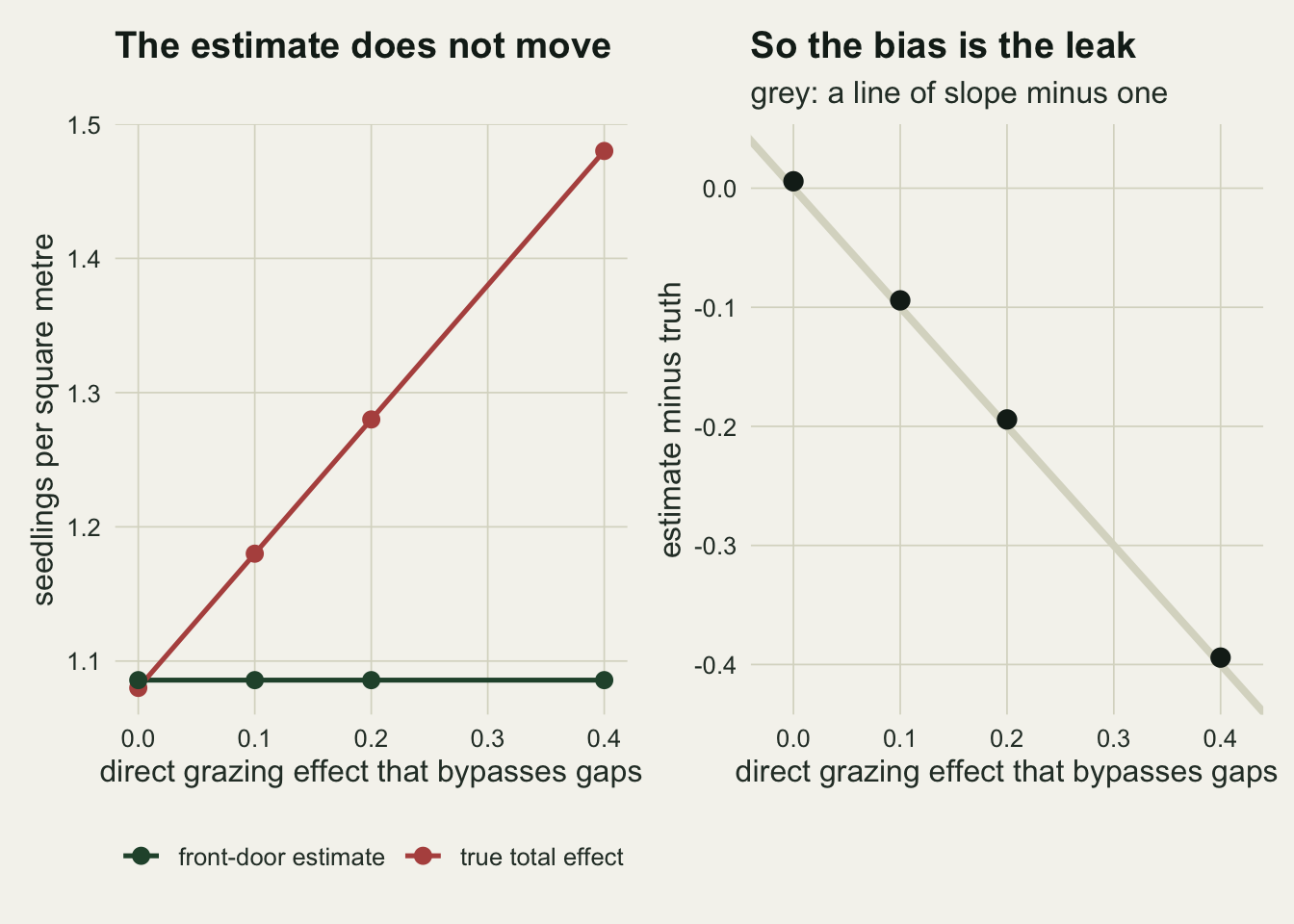
At a direct effect of one fifth of a seedling per square metre the front-door estimate is 15.2 per cent low, and at two fifths it is 26.6 per cent low. That price list is the whole sensitivity analysis for this method, and it is unusually easy to reason about: an ecologist who is prepared to say that trampling and dung dispersal together move recruitment by no more than some amount has thereby bounded the bias by that amount.
The next thing to want is a test, and a tempting one is to add a measured covariate to the second regression and read a significant coefficient as evidence that gap area does not carry everything. That test does not do what it looks like it does, and a counter-example built from the post’s own generating process settles it.
n_probe <- 400; n_prep <- 500; probe_leak <- 0.3; alpha_lev <- 0.05
probe_mcse <- 100 * sqrt(alpha_lev * (1 - alpha_lev) / n_prep)

probe_run <- function(via_dung, via_graze, rain_effect) {
  fert  <- rnorm(n_probe); rain <- rnorm(n_probe)
  graze <- g_ux * fert + rnorm(n_probe)
  gap   <- a_gap * graze + rnorm(n_probe)
  dung  <- 0.7 * graze + rnorm(n_probe)      # descendant of grazing, not of gap
  seedl <- b_rec * gap + via_dung * dung + via_graze * graze + rain_effect * rain +
           g_uy * fert + rnorm(n_probe)
  pv <- summary(lm(seedl ~ gap + graze + dung + rain))$coefficients[c("dung", "rain"), 4]
  c(p_dung = pv[[1]], p_rain = pv[[2]],
    fd = coef(lm(gap ~ graze))[["graze"]] * coef(lm(seedl ~ gap + graze))[["gap"]])
}

probe_rate <- function(via_dung, via_graze, rain_effect) {
  out <- replicate(n_prep, probe_run(via_dung, via_graze, rain_effect))
  c(rej_dung = 100 * mean(out["p_dung", ] < alpha_lev),
    rej_rain = 100 * mean(out["p_rain", ] < alpha_lev), fd = mean(out["fd", ]))
}

set.seed(7740)
probe_rain <- probe_rate(0, 0, 0.8)         # as drawn, plus a rainfall effect
probe_seen <- probe_rate(probe_leak, 0, 0)  # a leak running through dung
probe_hid  <- probe_rate(0, probe_leak, 0)  # a leak bypassing dung
Rainfall in that simulation is an ordinary independent cause of establishment with no link to grazing at all, so the front-door graph is exactly as drawn. Its coefficient in the second regression is significant at the five per cent level in 100.0 per cent of 500 surveys, while the front-door estimate on those surveys averages 1.082 against a truth of 1.08. Any cause of the outcome predicts the outcome after conditioning on the mediator, so the test fires on a graph it was meant to clear. A measured confounder of grazing and recruitment would fire it too.
The version that carries information is narrower: the covariate has to be a descendant of the treatment that is not a descendant of the mediator. Dung deposition is one. On those same surveys, where the graph is as drawn, dung is significant in 6.0 per cent of them, against a nominal five per cent with a Monte Carlo standard error of about 1.0 points. Route a direct effect of 0.3 through dung and it rises to 99.4 per cent. Route a bypass with the same coefficient straight from grazing so that it does not pass through dung, and dung falls back to 4.0 per cent while the estimate is biased all the same: 1.084 against a truth of 1.38. The check tests one named bypass route at a time. It is not a test of complete mediation, and there is no cheap test of complete mediation.
A weak mechanism costs precision, not validity
An instrument has to be strong. The 2SLS estimate divides the reduced-form slope by the first-stage slope, so a weak first stage puts a small noisy number in a denominator, and the estimate acquires a heavy tail and drifts back towards the confounded slope. The front-door estimator multiplies instead of dividing. The comparison is worth measuring because the intuition transfers badly, but only if the two sweeps ask the same question. Weakening the mechanism while leaving the gap-to-recruitment coefficient alone would shrink the estimand itself, and a shrinking target makes any absolute width fall for reasons that have nothing to do with the estimator. So the total effect is pinned at 1.08 in both sweeps: as the grazing-to-gap coefficient falls, the gap-to-recruitment coefficient is raised to compensate, exactly as the instrument sweep holds the causal effect fixed while the instrument weakens.
n_sweep <- 300; quart <- c(0.25, 0.5, 0.75)
str_set <- c(0.05, 0.1, 0.2, 0.4, 0.8, 1.2)

set.seed(3310)
fd_sweep <- as.data.frame(t(vapply(str_set, function(a) {
  reps <- replicate(n_sweep, front_door(sim_plots(n_plot, a, eff_true / a)))
  qq <- quantile(reps, quart)
  c(strength = a, truth = eff_true, lo = qq[[1]], med = qq[[2]], hi = qq[[3]])
}, numeric(5))))
fd_sweep$width <- fd_sweep$hi - fd_sweep$lo; fd_sweep$relw <- fd_sweep$width / eff_true

set.seed(3311)
iv_sweep <- as.data.frame(t(vapply(str_set, function(cz) {
  reps <- replicate(n_sweep, {
    fert  <- rnorm(n_plot); inst <- rnorm(n_plot)
    graze <- cz * inst + g_ux * fert + rnorm(n_plot)
    gap   <- a_gap * graze + rnorm(n_plot)
    seedl <- b_rec * gap + g_uy * fert + rnorm(n_plot)
    cov(inst, seedl) / cov(inst, graze)
  })
  qq <- quantile(reps, quart)
  c(strength = cz, truth = eff_true, lo = qq[[1]], med = qq[[2]], hi = qq[[3]])
}, numeric(5))))
iv_sweep$width <- iv_sweep$hi - iv_sweep$lo; iv_sweep$relw <- iv_sweep$width / eff_true

weakest <- 1; strongest <- length(str_set)
fd_rel_ratio <- fd_sweep$relw[weakest] / fd_sweep$relw[strongest]
iv_rel_ratio <- iv_sweep$relw[weakest] / iv_sweep$relw[strongest]
iv_drift <- iv_sweep$med[weakest] / eff_true; naive_ratio <- naive_mean / eff_true
fd_ratio_lo  <- min(fd_sweep$med) / eff_true; fd_ratio_hi <- max(fd_sweep$med) / eff_true
b_weakest    <- eff_true / str_set[weakest]
Both designs lose precision as they weaken. As the grazing-to-gap coefficient falls from 1.2 to 0.05, the interquartile width of the front-door estimate grows from 0.117 to 0.990, a factor of 8.4. The same sweep on instrument strength grows from 0.098 to 2.019, a factor of 20.5. The difference is in the centre, not the width. The front-door median sits between 0.98 and 1.03 times the truth across the whole range, which is inside the Monte Carlo noise of 300 replicates. The instrument median drifts to 1.28 times the truth at the weakest setting, part of the way back to the naive slope at 1.50 times the truth. Dividing by a number near zero moves the estimate as well as spreading it; multiplying by a small number only spreads it.
scaled_band <- function(tab) data.frame(strength = tab$strength,
  med = tab$med / tab$truth, lo = tab$lo / tab$truth, hi = tab$hi / tab$truth)
fd_band <- scaled_band(fd_sweep); iv_band <- scaled_band(iv_sweep)

band_panel <- function(tab, shade, panel_title, panel_sub, xlab) {
  ggplot(tab, aes(strength, med)) +
    geom_ribbon(aes(ymin = lo, ymax = hi), fill = shade, alpha = 0.25) +
    geom_hline(yintercept = 1, linetype = "dashed", colour = te_ink, linewidth = 0.6) +
    geom_line(colour = shade, linewidth = 0.9) +
    scale_x_log10() + coord_cartesian(ylim = c(0, 2.4)) +
    labs(x = xlab, y = "estimate as a multiple of the truth",
         title = panel_title, subtitle = panel_sub) +
    theme_datasheet()
}

p_fd <- band_panel(fd_band, te_forest, "Front-door: multiply",
  "band: interquartile range", "grazing to gap coefficient")
p_iv <- band_panel(iv_band, te_rust, "Instrument: divide",
  "dotted: the naive slope", "instrument to grazing coefficient") +
  geom_hline(yintercept = naive_ratio, linetype = "dotted", colour = te_gold,
             linewidth = 0.8)

p_fd + p_iv + plot_annotation(theme = theme_datasheet())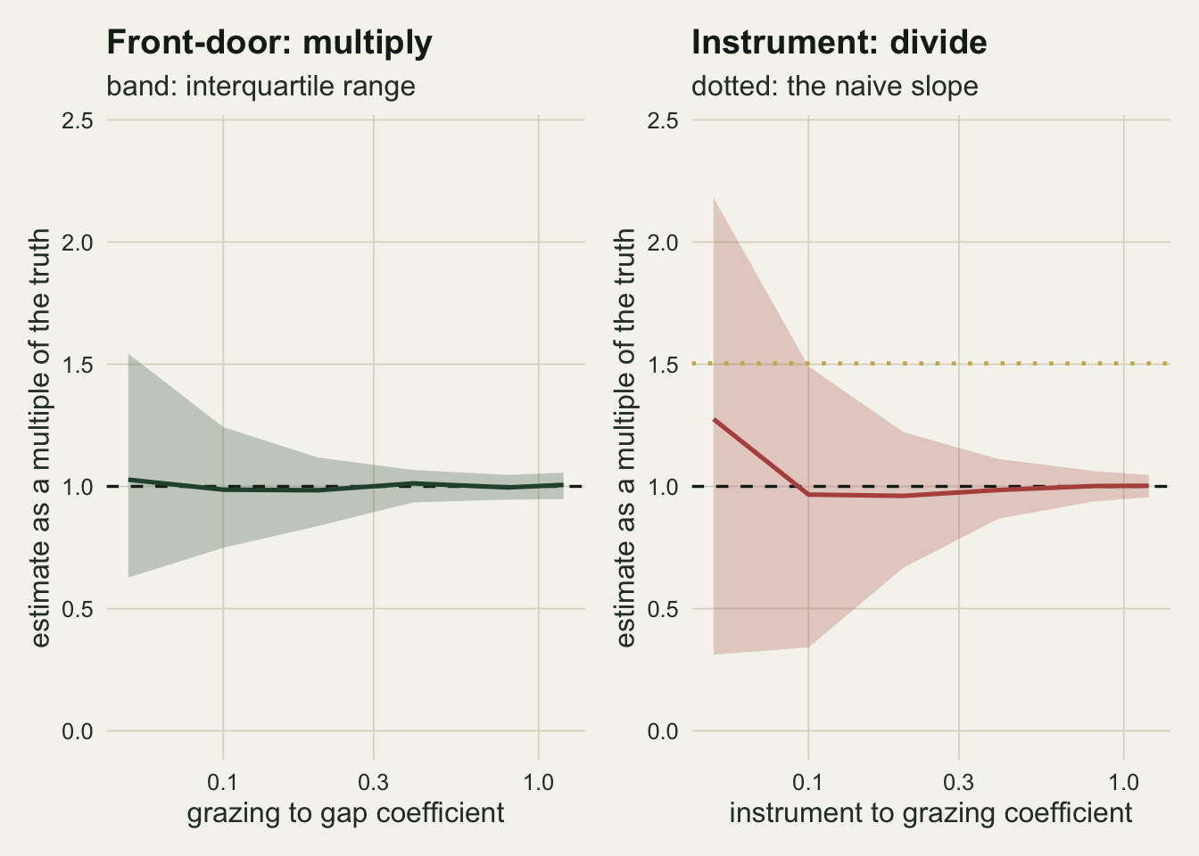
Neither panel makes weakness free. At the weakest setting the front-door interquartile range spans 92 per cent of the effect it is trying to measure, against 11 per cent at the strongest, so a weak mechanism buys a wide interval that still brackets the answer. The instrument case needs a first-stage rule of thumb and the front-door case does not, because only on the right does weakness move the number rather than blur it. One caveat about how the sweep was built: holding the total effect fixed while the mechanism weakens means raising the gap-to-recruitment coefficient to 21.6 at the far left, which is arithmetic rather than grassland ecology. In a real survey a mechanism that carries little of the grazing signal usually also means a small total effect, so the two difficulties arrive together: a wide interval, and not much inside it worth finding.
What to report
State the mediating mechanism as a claim about the system before showing any estimate, and say why the treatment could not reach the outcome by another route. That sentence is the whole identification argument, and a reader who does not accept it should not read the number that follows.
Report both stages, not only their product. The coefficient of the treatment on the mediator and the coefficient of the mediator on the outcome adjusted for treatment each have their own interpretation and their own standard error, and a reader who disagrees with one of them can recompute the total.
Give an interval, and say which regime it was checked in. The delta-method interval landed within a few tenths of nominal in the simulation above, where both coefficients were estimated sharply, and gave up about 2.4 percentage points of coverage in a small survey with two weakly estimated paths. A percentile bootstrap did not recover that in the paired comparison, so where both paths are weak the answer is a larger survey rather than a different formula.
Publish a leakage table. Pick two or three plausible sizes for the direct effect, state what each implies for the total, and let the reader see that the bias is subtraction rather than something that has to be simulated. Glynn and Kashin (2018) give the general bias formulas for the front-door estimand and for hybrid estimators that use partial adjustment alongside it.
Be precise about what any check on the graph can see. A covariate that predicts the outcome after conditioning on the mediator and the treatment is not evidence against complete mediation: rainfall does that on a graph with no direct path in it. A descendant of the treatment that is not a descendant of the mediator is the version that carries information, and even that only rules out the one bypass route it names. Complete mediation has no cheap data-side check, so the sentence that asserts it is where the effort belongs.
Honest limits
Complete mediation is not testable from these data. Bellemare, Bloem and Wexler (2024) work through a single application chosen because the assumptions plausibly hold there, whether deciding to share an Uber or Lyft ride changes tipping, and set out the identification and estimation machinery around it; the consequences of violating the assumptions are explored in their appendix rather than in the headline result. The leakage sweep above is the price list for that failure, and it is the most useful thing this post produces: an ecologist who cannot rule out trampling can still bound the bias by the size of the trampling effect, which is a smaller claim than ruling it out.
The formula assumes no unmeasured confounding of the mediator with the outcome either. In this grassland that means nothing may drive both gap area and seedling recruitment other than grazing and what is already in the model, and small-scale soil disturbance, ant nests, mole hills and rabbit scrapes all violate it. That assumption is often as strong as the one front-door adjustment was brought in to avoid, so an application stands or falls on whether the mediator’s own confounding is easier to argue away than the treatment’s, which is a judgement about the system and not about the method.
Everything here is linear, additive and Gaussian, which is what lets the general formula collapse to a product of two coefficients. With a count outcome, a saturating mediator response or an interaction between grazing and gap area, the product is no longer the front-door estimand and the two-stage averaging has to be done as written, by simulation from the fitted models. Arif and MacNeil (2023) set out the structural causal model framework for ecology in the general form, and that is where the non-linear version of this argument belongs.
The mediator is treated as measured without error. Gap area estimated by point quadrat or from photographs carries substantial error, and attenuation in the mediator biases the gap-to-recruitment coefficient towards zero, which propagates straight into the product. Unlike leakage, that bias is multiplicative and it does interact with everything else in the model.
The simulation uses 500 surveys for the main comparison, 20000 for each of the three long-run coverage regimes, 300 per point in the strength sweeps and 1500 for the paired delta and bootstrap comparison, so the sweep quartiles carry visible Monte Carlo noise while the long-run coverage figures are pinned to about 0.16 of a percentage point. Sizing those runs matters more than it looks. The 93.6 per cent the main study returned sits 1.4 Monte Carlo standard errors from nominal, which is an ordinary draw, and only the longer run can separate that from a shortfall worth acting on. The leakage identity carries no Monte Carlo noise at all, since it holds within each replicate exactly.
References
Pearl J 1995 Biometrika 82(4):669-688 (10.1093/biomet/82.4.669)
Pearl J 2009 Causality: Models, Reasoning and Inference, 2nd ed. Cambridge University Press (ISBN 978-0-521-89560-6)
Glynn AN, Kashin K 2018 Journal of the American Statistical Association 113(523):1040-1049 (10.1080/01621459.2017.1398657)
Bellemare MF, Bloem JR, Wexler N 2024 Oxford Bulletin of Economics and Statistics 86(4):951-993 (10.1111/obes.12598)
Arif S, MacNeil MA 2023 Ecological Monographs 93(1):e1554 (10.1002/ecm.1554)
Larsen AE, Meng K, Kendall BE 2019 Methods in Ecology and Evolution 10(7):924-934 (10.1111/2041-210X.13190)