Attrition in a field experiment: when pots die first

When a treatment changes which pots survive to harvest, the survivor contrast is not the effect. Lee bounds, Imbens-Manski intervals and the survival gap in R.

Six hundred pots of a native forb, half of them given a slow-release fertiliser at sowing, go through a dry summer on an unwatered bench. In September the survivors are clipped, dried and weighed. The fertilised pots have many more survivors than the controls, and the obvious analysis compares the mean dry mass of the surviving fertilised pots with the mean of the surviving controls, with a two-sample interval. The randomisation was clean, the harvest was blind, and the contrast still does not estimate what the fertiliser does to a plant.

The reason is who is being compared. A control pot survives the drought only if its seedling was vigorous. A fertilised pot survives if it was vigorous, or if it was middling and the fertiliser carried it through. The fertilised survivors therefore include weaker plants that the control arm lost, and weaker plants grow less. Randomisation made the two arms alike at sowing; the drought made the two sets of survivors unlike at harvest, and the difference between them is caused by the treatment. The same shape turns up in mesocosm trials where tanks crash, in toxicity assays scored only on survivors, in transplant experiments measured on the plants that established, and in any seedling trial with a growth response.

The non-compliance post keeps the unit and loses the treatment. Non-compliance in field experiments has a fence that fails on some plots, and every plot is still measured; the repair there is to divide by the compliance rate. Here the unit is gone, randomisation survives the assignment and dies at the harvest, and the only valid answer is an interval that no standard error produces and that is usually too wide to be worth having: which is itself the result, and the number to report with it is the survival gap. (The width of that interval comes from the survival rates and the spread of the harvest, not from a standard error; the sampling error has to be added on top, as the Imbens-Manski section shows.)

The mechanism has names elsewhere on this site. Collider bias and selection shows that sampling on a common effect manufactures an association, but its setting is observational and its repair is not to condition on the collider. In a pot trial there is no such choice, because a dead pot has no biomass to weigh. Checking a monitoring design measures what selective loss of sites does to a trend and finds that loss tied to the state of the site moves the estimate most of the way to zero, without offering a repair. The nearest thing on the site to a bracket instead of a point estimate is in Lost collar signals and informative censoring, whose report section asks for two Kaplan-Meier curves, one treating lost collars as censored and one treating them as deaths, and reads the pair as a bracket. That is a worst-case bracket on a survival curve. What follows is a bracket on a treatment contrast, built from the one assumption a randomised experiment can offer. It also differs from Missing values in a predictor, where the reason for a blank decides between two estimators that already exist; here the treatment itself decides which values go missing, and no estimator is right. And it is a different failure from Interference between experimental plots, where every plot is measured but a treated plot leaks into its neighbours.

None of the method is new. Horowitz and Manski 2000 gave worst-case bounds for randomised experiments with missing outcomes. Zhang and Rubin 2003 named the quantity that survives the problem, the effect among units that would have lived under either treatment, and called the problem truncation by death, which is a pot trial exactly. Lee 2009 showed that under one assumption the bounds on that quantity can be made sharp by trimming. Imbens and Manski 2004 gave the confidence interval that goes with a bound. This post is a demonstration of their results on a simulated pot trial, not a claim to any of them. What it measures is how fast the survivor interval stops covering as the survival gap widens, how wide the honest bound is at the same gaps, and what happens at the two edges: a fertiliser with no effect on survival, and a fertiliser that kills some seedlings that would otherwise have lived.

What the survivors can and cannot say

Every pot has two potential fates, alive or dead at harvest with the fertiliser and alive or dead without it, and only one is observed. That splits the pots into strata that randomisation cannot see: pots that would survive either way, pots that survive only if fertilised, pots that die either way, and, if the fertiliser can ever kill, pots that survive only without it. Zhang and Rubin 2003 point out that a harvest effect is only defined for the first group, since the others have no harvest in at least one arm. Their estimand is the effect among the always-survivors.

The control survivors are always-survivors, if the fertiliser never kills a pot that would have lived. That condition is monotonicity, and it is an assumption, not a fact about fertiliser: a salt-heavy dose that scorches the roots of weak seedlings breaks it, and a section below measures what happens then. Under monotonicity the fertilised survivors are a mixture of always-survivors and pots rescued by the fertiliser, and the rescued share is known from the two survival rates. If the survival rates are s1 for fertilised and s0 for control, the share of fertilised survivors that were rescued is (s1 - s0) / s1. The denominator is s1, the surviving share of the fertilised arm, not the whole arm and not one: dividing by anything else trims the wrong number of plants.

Which of the fertilised survivors were rescued is not known. The worst case for the effect is that the rescued plants were the heaviest, and the best case is that they were the lightest. Lee 2009 turns that into two numbers. Drop the heaviest (s1 - s0) / s1 of the fertilised survivors and compare the rest with the controls, which gives the lower bound; drop the lightest share instead, which gives the upper bound. The bound endpoints are arithmetic: given the two survival rates, the harvest distribution of the fertilised survivors and the mean of the control survivors, they follow from the trimming rule with no model and no estimate of anything. The rest of this post is about what the arithmetic does in repeated trials.

Six hundred pots and a vigour nobody measured

The simulation gives each pot a latent vigour that nobody records. Vigour raises the chance of surviving the drought and raises the harvest. The fertiliser shifts survival on the logit scale by an amount that is swept below, and adds a fixed amount to the log dry mass of every pot, so the effect among always-survivors, the effect among all pots, and the effect on any subgroup are one number. That is deliberate: it removes every question about which estimand is meant, and leaves only the selection.

library(ggplot2)
library(patchwork)

te_paper  <- "#f5f4ee"
te_ink    <- "#16241d"
te_body   <- "#2c3a31"
te_forest <- "#275139"
te_rust   <- "#b5534e"
te_gold   <- "#c9b458"
te_line   <- "#dad9ca"

theme_datasheet <- function() {
  theme_minimal(base_size = 12) +
    theme(plot.background  = element_rect(fill = te_paper, colour = NA),
          panel.background = element_rect(fill = te_paper, colour = NA),
          panel.grid.major = element_line(colour = te_line, linewidth = 0.3),
          panel.grid.minor = element_blank(),
          text             = element_text(colour = te_body),
          plot.title       = element_text(colour = te_ink, face = "bold"),
          plot.subtitle    = element_text(colour = te_body),
          axis.text        = element_text(colour = te_body))
}

a0       <- -0.20   # survival intercept (logit), control arm
s_q      <- 1.0     # vigour loading in survival
b_q      <- 1.2     # vigour loading in the harvest
mu0      <- 2       # mean log dry shoot mass, control
tau_true <- 0.50    # effect of the fertiliser on log mass, every pot
d_grid   <- c(0, 0.6, 1.2, 1.8, 2.4, 3.0)   # fertiliser effect on survival (logit)
n_grid   <- c(200, 600)                     # pots per trial, split 1:1
tau_grid <- c(-0.50, 0, 0.50)
n_rep    <- 1000                            # fresh trials per cell, fixed in advance

grow_pots <- function(n_pots, d, tau, cut = -Inf) {
  z     <- rep(0:1, each = n_pots / 2)
  q     <- rnorm(n_pots)                          # latent vigour, never recorded
  u     <- runif(n_pots)                          # one draw per pot: fixes who lives
  alive <- u < plogis(a0 + d * z + s_q * q)
  alive <- alive & !(z == 1 & q < cut)            # burn arm only: weak treated pots die
  y     <- mu0 + tau * z + b_q * q + rnorm(n_pots) # harvest, seen only if alive
  list(z = z, alive = alive, y = y)
}

A pot survives if its uniform draw falls below its survival probability, and the same draw serves both arms, so the fertiliser can only move a pot from dead to alive: monotonicity holds by construction until the cut argument is used. The harvest is generated for every pot and then thrown away for the dead ones, which is the only way to know the truth for a quantity that the experiment never sees.

The analysis has three parts. The survivor contrast is a Welch two-sample interval on the survivors. The Lee bound trims the arm with the higher survival, which is the fertilised arm whenever the fertiliser helps. Its standard errors follow Lee 2009: a trimmed-mean term, a term for having estimated the trim share, and a term for the other arm’s mean. The Imbens-Manski interval widens each end of the bound by a multiple of its own standard error, with the multiple chosen so that the true effect, wherever it sits inside the bound, is covered at 95 per cent; the multiple is 1.96 when the bound has no width and falls towards 1.645 as the bound becomes wide relative to its standard errors.

trim_side <- function(ys, p_trim, keep) {
  m <- length(ys); k <- max(2, round((1 - p_trim) * m))
  kept <- if (keep == "low") ys[1:k] else ys[(m - k + 1):m]
  xi   <- if (keep == "low") ys[k] else ys[m - k + 1]
  mu   <- mean(kept)
  list(mu = mu, v_trim = (var(kept) + p_trim * (xi - mu)^2) / ((1 - p_trim) * m),
       slope = (mu - xi) / (1 - p_trim))
}

im_crit <- function(width, se_max, level = 0.95) {
  r <- width / se_max
  if (r > 40) return(qnorm(level))
  uniroot(function(cc) pnorm(cc + r) - pnorm(-cc) - level, c(0, 3), tol = 1e-9)$root
}

analyse_trial <- function(pots) {
  n1 <- sum(pots$z == 1); n0 <- sum(pots$z == 0)
  y1 <- sort(pots$y[pots$alive & pots$z == 1]); y0 <- sort(pots$y[pots$alive & pots$z == 0])
  m1 <- length(y1); m0 <- length(y0); s1 <- m1 / n1; s0 <- m0 / n0
  v1 <- var(y1); v0 <- var(y0)
  se_w  <- sqrt(v1 / m1 + v0 / m0)
  df_w  <- se_w^4 / ((v1 / m1)^2 / (m1 - 1) + (v0 / m0)^2 / (m0 - 1))
  naive <- mean(y1) - mean(y0)
  half  <- qt(0.975, df_w) * se_w
  if (s1 >= s0) {                                   # trim the fertilised survivors
    p_trim <- (s1 - s0) / s1
    v_p <- s0 * (1 - s0) / (n0 * s1^2) + s0^2 * (1 - s1) / (n1 * s1^3)
    a <- trim_side(y1, p_trim, "low"); b <- trim_side(y1, p_trim, "high")
    lo <- a$mu - mean(y0); hi <- b$mu - mean(y0); v_other <- v0 / m0
  } else {                                          # trim the control survivors
    p_trim <- (s0 - s1) / s0
    v_p <- s1 * (1 - s1) / (n1 * s0^2) + s1^2 * (1 - s0) / (n0 * s0^3)
    a <- trim_side(y0, p_trim, "high"); b <- trim_side(y0, p_trim, "low")
    lo <- mean(y1) - a$mu; hi <- mean(y1) - b$mu; v_other <- v1 / m1
  }
  se_lo <- sqrt(a$v_trim + a$slope^2 * v_p + v_other)
  se_hi <- sqrt(b$v_trim + b$slope^2 * v_p + v_other)
  cc <- im_crit(hi - lo, max(se_lo, se_hi))
  c(s0 = s0, s1 = s1, p_trim = p_trim, naive = naive,
    n_lo = naive - half, n_hi = naive + half, lo = lo, hi = hi,
    se_lo = se_lo, se_hi = se_hi, im_lo = lo - cc * se_lo, im_hi = hi + cc * se_hi)
}

run_cell <- function(n_pots, d, tau, cut = -Inf, reps = n_rep)
  t(replicate(reps, analyse_trial(grow_pots(n_pots, d, tau, cut))))
covers <- function(lo, hi, truth) mean(lo <= truth & truth <= hi)

One season, trimmed by hand

One trial with 600 pots and a fertiliser that raises survival strongly, d = 1.8 on the logit scale, shows every step.

set.seed(2718)
pots_one <- grow_pots(600, 1.8, tau_true)
one <- analyse_trial(pots_one)
y1_one <- pots_one$y[pots_one$alive & pots_one$z == 1]
y0_one <- pots_one$y[pots_one$alive & pots_one$z == 0]
welch_gap <- max(abs(t.test(y1_one, y0_one)$conf.int - one[c("n_lo", "n_hi")]))
k_drop <- length(y1_one) - max(2, round((1 - one[["p_trim"]]) * length(y1_one)))
round(one, 3)

    s0     s1 p_trim  naive   n_lo   n_hi     lo     hi  se_lo  se_hi  im_lo 
 0.503  0.823  0.389  0.171 -0.129  0.471 -0.810  1.158  0.183  0.187 -1.111 
 im_hi 
 1.465 

Of the 300 control pots, 151 survived, a rate of 0.503; of the fertilised pots, 247 survived, 0.823. The survival gap is 0.320, and the share of fertilised survivors to trim is that gap divided by 0.823, which is 0.389: 96 plants from one end or the other.

The survivor contrast is +0.171 log units with a Welch interval from -0.129 to +0.471. The hand-coded interval agrees with the one from t.test to within floating-point rounding. The true effect is 0.50, and it is outside that interval. Trimming the heaviest 96 fertilised survivors gives a lower bound of -0.810; trimming the lightest gives an upper bound of +1.158. The Imbens-Manski interval runs from -1.111 to +1.465.

ord1 <- sort(y1_one)
n_keep <- length(ord1) - k_drop
tag1 <- ifelse(seq_along(ord1) > n_keep, "cut for lower bound",
         ifelse(seq_along(ord1) <= k_drop, "cut for upper bound", "kept by both"))
strip_df <- rbind(
  data.frame(arm = "control", y = y0_one, trim = "control"),
  data.frame(arm = "fertilised", y = ord1, trim = tag1))
strip_df$trim <- factor(strip_df$trim, levels = c("control", "kept by both",
  "cut for upper bound", "cut for lower bound"))
set.seed(11)
strip_df$jit <- as.numeric(factor(strip_df$arm)) + runif(nrow(strip_df), -0.28, 0.28)
p_strip <- ggplot(strip_df, aes(y, jit, colour = trim)) +
  geom_point(aes(shape = trim), size = 1.2, alpha = 0.85, stroke = 0.5) +
  scale_colour_manual(values = c(te_body, te_forest, te_gold, te_rust), name = NULL) +
  scale_shape_manual(values = c(1, 16, 16, 16), name = NULL) +
  scale_y_continuous(breaks = 1:2, labels = c("control", "fertilised")) +
  guides(colour = guide_legend(nrow = 2, override.aes = list(size = 2.5)),
         shape = guide_legend(nrow = 2)) +
  labs(x = "log dry shoot mass", y = NULL, title = "Survivors at harvest",
       subtitle = "one trial, 600 pots") +
  theme_datasheet() + theme(legend.position = "bottom")

iv_df <- data.frame(
  what = factor(c("survivor contrast", "Lee bound", "Imbens-Manski"),
                levels = rev(c("survivor contrast", "Lee bound", "Imbens-Manski"))),
  lo = c(one[["n_lo"]], one[["lo"]], one[["im_lo"]]),
  hi = c(one[["n_hi"]], one[["hi"]], one[["im_hi"]]),
  mid = c(one[["naive"]], NA, NA))
p_iv <- ggplot(iv_df, aes(y = what, colour = what)) +
  geom_vline(xintercept = tau_true, colour = te_ink, linetype = "dashed", linewidth = 0.6) +
  geom_errorbar(aes(xmin = lo, xmax = hi), orientation = "y", width = 0.25, linewidth = 1) +
  geom_point(aes(x = mid), size = 2.6, na.rm = TRUE) +
  scale_colour_manual(values = c(te_gold, te_forest, te_rust), guide = "none") +
  labs(x = "effect on log dry shoot mass", y = NULL, title = "Three answers",
       subtitle = "dashed line: the true effect") +
  theme_datasheet()

p_strip + p_iv + plot_layout(widths = c(1.4, 1)) + plot_annotation(theme = theme_datasheet())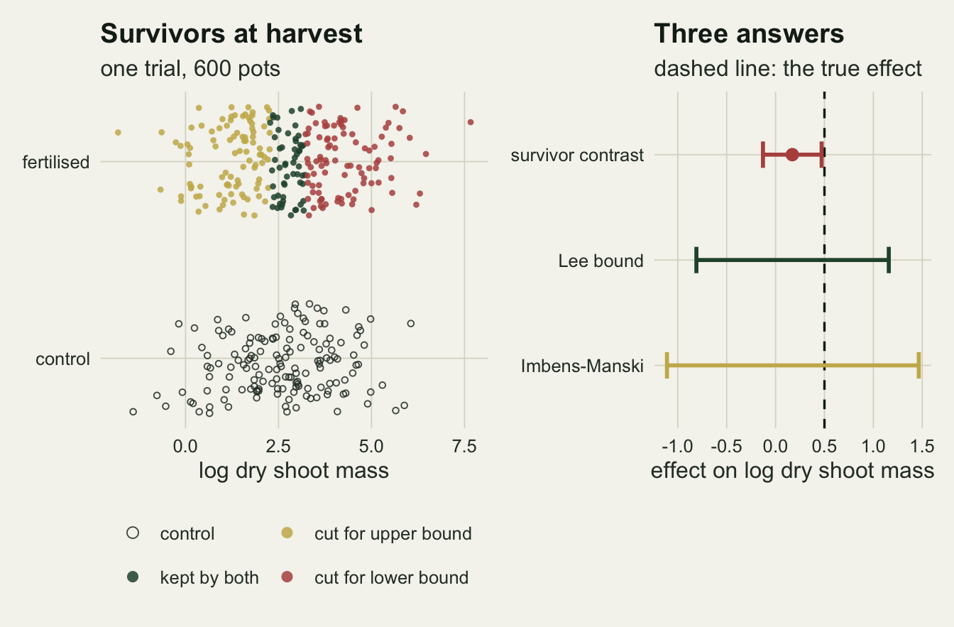

Figure 1: One simulated pot trial. Left: harvest of every surviving pot, with the fertilised survivors coloured by the trim they fall in. Right: the survivor contrast, the Lee bound and the Imbens-Manski interval against the true effect.

The bound is arithmetic before it is statistics

Everything in the previous section has a population value that needs no simulation. Vigour is normal and the survival curve is logistic, so the survivors of each arm have a harvest distribution that is a mixture of normals, weighted by how likely each vigour was to survive. A quadrature over vigour gives both survival rates, the value the survivor contrast converges to, and both endpoints of the bound, for an infinitely large trial.

q_nodes <- seq(-8, 8, length.out = 4001)
q_w     <- dnorm(q_nodes) * diff(q_nodes[1:2])
arm_mix <- function(d, tau, z, cut = -Inf) {
  pa <- plogis(a0 + d * z + s_q * q_nodes) * (if (z == 1) q_nodes >= cut else 1)
  s  <- sum(q_w * pa)
  list(s = s, w = q_w * pa / s, m = mu0 + tau * z + b_q * q_nodes)
}
mix_cdf   <- function(mx, yv) sum(mx$w * pnorm(yv - mx$m))
mix_below <- function(mx, yv) sum(mx$w * (mx$m * pnorm(yv - mx$m) - dnorm(yv - mx$m)))
mix_mean  <- function(mx) sum(mx$w * mx$m)
mix_trim  <- function(mx, g, keep) {
  if (g > 1 - 1e-9) return(mix_mean(mx))
  target <- if (keep == "low") g else 1 - g
  yq <- uniroot(function(yv) mix_cdf(mx, yv) - target, c(-15, 20), tol = 1e-10)$root
  if (keep == "low") mix_below(mx, yq) / g else (mix_mean(mx) - mix_below(mx, yq)) / g
}
pop_trial <- function(d, tau, cut = -Inf) {
  m0 <- arm_mix(d, tau, 0); m1 <- arm_mix(d, tau, 1, cut)
  if (m1$s >= m0$s) {
    p_trim <- (m1$s - m0$s) / m1$s
    lo <- mix_trim(m1, 1 - p_trim, "low") - mix_mean(m0)
    hi <- mix_trim(m1, 1 - p_trim, "high") - mix_mean(m0)
  } else {
    p_trim <- (m0$s - m1$s) / m0$s
    lo <- mix_mean(m1) - mix_trim(m0, 1 - p_trim, "high")
    hi <- mix_mean(m1) - mix_trim(m0, 1 - p_trim, "low")
  }
  c(s0 = m0$s, s1 = m1$s, gap = m1$s - m0$s, p_trim = p_trim,
    naive = mix_mean(m1) - mix_mean(m0), lo = lo, hi = hi)
}
pop <- as.data.frame(t(sapply(d_grid, function(d) pop_trial(d, tau_true))))
pop$d <- d_grid; pop$bias <- pop$naive - tau_true; pop$width <- pop$hi - pop$lo
pop_harm <- pop_trial(2.4, -tau_true)
round(pop, 3)

     s0    s1   gap p_trim naive     lo    hi   d   bias width
1 0.459 0.459 0.000  0.000 0.500  0.500 0.500 0.0  0.000 0.000
2 0.459 0.582 0.123  0.212 0.379 -0.168 0.923 0.6 -0.121 1.091
3 0.459 0.697 0.238  0.342 0.269 -0.566 1.102 1.2 -0.231 1.667
4 0.459 0.793 0.334  0.422 0.177 -0.844 1.197 1.8 -0.323 2.040
5 0.459 0.866 0.408  0.471 0.106 -1.039 1.249 2.4 -0.394 2.288
6 0.459 0.918 0.459  0.500 0.053 -1.171 1.278 3.0 -0.447 2.449

Without the fertiliser 0.459 of the pots survive. Across the sweep the fertilised survival rises from the same value to 0.918, so the survival gap runs from zero to 0.459. The survivor contrast converges to 0.379 at the smallest nonzero gap and to 0.053 at the largest, against a true effect of 0.50: a bias from -0.121 to -0.447 that no amount of replication removes, because it is the value the estimator is consistent for. The fertilised survivors include rescued plants of lower vigour, vigour raises the harvest, and so the bias is downward.

The bound endpoints at infinite sample size are -0.168 and +0.923 at the smallest nonzero gap and -1.171 and +1.278 at the largest. The width grows from 1.09 to 2.45 log units, 2.2 to 4.9 times the effect it is bounding. These are the identified sets: the range of effects consistent with the survival rates and the survivor distributions, and nothing a larger trial can narrow. The true effect lies well inside every one of them. That is a feature of this design and not a guarantee; it matters for how the coverage figures below should be read.

A thousand trials along the survival gap

Now the sampling. Each cell of the grid runs 1000 fresh trials, a number fixed before anything was inspected. Coverage below is the share of those 1000 trials whose interval contains the true effect: it is out of trials, never out of pots, and its Monte Carlo standard error is at most 0.016.

set.seed(40961)
cells <- expand.grid(d = d_grid, tau = tau_grid, n_pots = n_grid)
sims <- lapply(seq_len(nrow(cells)), function(i)
  run_cell(cells$n_pots[i], cells$d[i], cells$tau[i]))
summ_cell <- function(R, tau, d) {
  pt <- pop_trial(d, tau)
  c(gap_obs = median(R[, "s1"] - R[, "s0"]), naive = median(R[, "naive"]),
    cov_naive = covers(R[, "n_lo"], R[, "n_hi"], tau),
    cov_own = covers(R[, "n_lo"], R[, "n_hi"], pt[["naive"]]),
    cov_lee = covers(R[, "lo"], R[, "hi"], tau),
    cov_im = covers(R[, "im_lo"], R[, "im_hi"], tau),
    lo = median(R[, "lo"]), hi = median(R[, "hi"]),
    width = median(R[, "hi"] - R[, "lo"]),
    im_lo = median(R[, "im_lo"]), im_hi = median(R[, "im_hi"]),
    im_width = median(R[, "im_hi"] - R[, "im_lo"]),
    n_lo = median(R[, "n_lo"]), n_hi = median(R[, "n_hi"]),
    n_width = median(R[, "n_hi"] - R[, "n_lo"]),
    sd_lo = sd(R[, "lo"]), se_lo = median(R[, "se_lo"]),
    sd_hi = sd(R[, "hi"]), se_hi = median(R[, "se_hi"]))
}
sweep <- cbind(cells, gap = pop$gap[match(cells$d, pop$d)],
  t(sapply(seq_len(nrow(cells)), function(i) summ_cell(sims[[i]], cells$tau[i], cells$d[i]))))
cell_of <- function(n_pots, tau) sweep[sweep$n_pots == n_pots & sweep$tau == tau, ]
main <- cell_of(600, tau_true); small <- cell_of(200, tau_true)
naive_drop <- main$cov_naive[1] - main$cov_naive[6]
lee_min_wide <- min(sweep$cov_lee[sweep$gap > 0.2])
own_range <- range(sweep$cov_own)
i_small <- which(cells$n_pots == 200 & cells$d == d_grid[2] & cells$tau == tau_true)
up_miss_small <- mean(sims[[i_small]][, "hi"] < tau_true)   # upper end below the truth
round(main[, c("gap", "naive", "cov_naive", "cov_lee", "cov_im", "width", "im_width")], 3)

     gap naive cov_naive cov_lee cov_im width im_width
31 0.000 0.490     0.954   0.600  1.000 0.342    1.350
32 0.123 0.378     0.894   0.964  0.999 1.085    1.808
33 0.238 0.267     0.691   1.000  1.000 1.663    2.312
34 0.334 0.179     0.478   1.000  1.000 2.033    2.657
35 0.408 0.115     0.316   1.000  1.000 2.278    2.892
36 0.459 0.055     0.193   1.000  1.000 2.449    3.053

At 600 pots the survivor interval covers the true effect in 0.954 of trials when the fertiliser does not touch survival. It covers 0.894 at a survival gap of 0.12, 0.691 at 0.24, 0.478 at 0.33, 0.316 at 0.41 and 0.193 at 0.46. It never reaches zero in this sweep, but by the widest gap it has fallen by 0.76 in absolute terms.

At 200 pots the same gaps give 0.937, 0.869, 0.790, 0.694 and 0.659. The smaller trial looks safer only because its interval is wider around the same wrong centre. The bias is a property of the gap, not of the sample size, so every extra pot narrows the interval around the wrong value: at a gap of 0.24 the trial of 600 pots covers 0.691 of the time and the trial of 200 covers 0.869.

The interval is not broken. Across all 36 cells it covers its own target, the population survivor contrast from the quadrature, in between 0.937 and 0.963 of trials. It is a correct interval for the mean mass of a surviving fertilised plant minus the mean mass of a surviving control plant. The error is in calling that the effect of the fertiliser.

sw_long <- rbind(
  data.frame(gap = main$gap, lo = main$n_lo, hi = main$n_hi, what = "survivor contrast, Welch interval"),
  data.frame(gap = main$gap, lo = main$lo, hi = main$hi, what = "Lee bound"),
  data.frame(gap = main$gap, lo = main$im_lo, hi = main$im_hi, what = "Imbens-Manski interval"))
sw_long$what <- factor(sw_long$what, levels = c("Imbens-Manski interval", "Lee bound",
                                                "survivor contrast, Welch interval"))
ggplot(sw_long, aes(gap)) +
  geom_ribbon(aes(ymin = lo, ymax = hi, fill = what), alpha = 0.55) +
  geom_line(aes(y = lo, colour = what), linewidth = 0.7) +
  geom_line(aes(y = hi, colour = what), linewidth = 0.7) +
  geom_line(data = main, aes(y = naive), colour = te_rust, linewidth = 1) +
  geom_hline(yintercept = tau_true, colour = te_ink, linetype = "dashed", linewidth = 0.7) +
  scale_fill_manual(values = c(te_gold, te_forest, te_rust), name = NULL) +
  scale_colour_manual(values = c(te_gold, te_forest, te_rust), name = NULL) +
  guides(fill = guide_legend(nrow = 2), colour = guide_legend(nrow = 2)) +
  labs(x = "survival gap, fertilised minus control", y = "effect on log dry shoot mass",
       title = "The survivor interval leaves the truth; the bound swallows it",
       subtitle = "dashed line: the true effect; medians over 1000 trials of 600 pots") +
  theme_datasheet() + theme(legend.position = "bottom")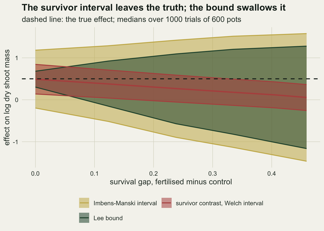

Figure 2: Median intervals from 1000 trials of 600 pots at each survival gap: the survivor contrast, the Lee bound and the Imbens-Manski interval, against the true effect.

The bound behaves the other way. Wherever the survival gap exceeds 0.2 it covers the true effect in at least 0.935 of trials, at both trial sizes. With 600 pots its median width is 1.08 log units at the smallest nonzero gap and 2.45 at the largest, so 2.2 to 4.9 times the true effect of 0.50; the Imbens-Manski interval adds sampling error and runs from 1.81 to 3.05. Those numbers carry the trade-off. The width grows with the gap, as the bias does, because both come from the same rescued plants. At a gap of 0.12, where the bound is narrowest among the nonzero gaps, the survivor interval still covers 0.894 of the time with 600 pots against the bound’s 0.964, so the bound buys a few points of coverage at a width 2.2 times the effect. At 200 pots the same gap is worse than that: the raw bound covers 0.830 against the survivor interval’s 0.937, because the truth is close enough to the upper end of the identified set for sampling error to push the end below it, which happens in 0.134 of those trials. At a gap of 0.46, where the survivor interval is hopeless, the bound spans every value from a loss of 1.16 log units to a gain of 1.28, and cannot even say whether the fertiliser helps or hurts growth.

A coverage of one here is not precision. Away from the smallest gaps the true effect sits well inside a wide identified set, so any interval that contains the set contains the truth. The coverage of a bound is only tested where the truth sits near one of its ends: at zero gap, in the next section, and in small trials at the smallest nonzero gap.

cov_long <- do.call(rbind, lapply(n_grid, function(nn) {
  tb <- cell_of(nn, tau_true)
  data.frame(gap = rep(tb$gap, 3), pots = sprintf("%d pots", nn),
             what = rep(c("survivor contrast", "Lee bound", "Imbens-Manski"), each = nrow(tb)),
             cover = c(tb$cov_naive, tb$cov_lee, tb$cov_im))
}))
cov_long$what <- factor(cov_long$what, levels = c("survivor contrast", "Lee bound", "Imbens-Manski"))
cov_long$pots <- factor(cov_long$pots, levels = sprintf("%d pots", n_grid))
cov_long$mcse <- sqrt(cov_long$cover * (1 - cov_long$cover) / n_rep)
ggplot(cov_long, aes(gap, cover, colour = what)) +
  geom_hline(yintercept = 0.95, colour = te_body, linetype = "dashed", linewidth = 0.5) +
  geom_errorbar(aes(ymin = cover - 2 * mcse, ymax = cover + 2 * mcse), width = 0.015,
                linewidth = 0.4) +
  geom_line(linewidth = 0.9) + geom_point(size = 2) +
  facet_wrap(~pots) +
  scale_colour_manual(values = c(te_rust, te_forest, te_gold), name = NULL) +
  scale_y_continuous(limits = c(0, 1)) +
  labs(x = "survival gap, fertilised minus control", y = "coverage of the true effect",
       title = "More pots make the survivor interval worse",
       subtitle = "dashed line: 95 per cent; 1000 trials per point") +
  theme_datasheet() + theme(legend.position = "bottom")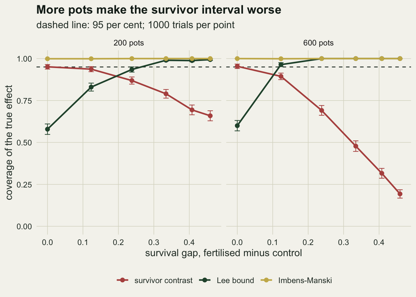

Figure 3: Coverage of the true effect by the three intervals across the survival gap, for trials of 200 and 600 pots, with two Monte Carlo standard errors.

With no survival effect the bound has no error bar

When the fertiliser does not change survival at all, the identified set is a single point: the survival rates are equal, nothing needs trimming, and the survivor contrast is the effect. A sample never shows equal survival rates, though. The estimated gap is positive or negative by chance, the arm that happens to look better gets trimmed by that chance amount, and the bound comes out as a narrow interval whose width reflects only the accidental gap. Nothing in the trimming rule accounts for the sampling error of the two means, so a narrow bound in the wrong place is reported with the same confidence as a wide one.

at0 <- sweep[sweep$d == 0 & sweep$tau == tau_true, ]
se_ratio <- c(sweep$se_lo / sweep$sd_lo, sweep$se_hi / sweep$sd_hi)   # both endpoints
d_ratio  <- c(sweep$d, sweep$d)
se_ratio_0 <- se_ratio[d_ratio == 0]; se_ratio_pos <- se_ratio[d_ratio > 0]
oracle_im <- function(R, tau) {
  sl <- sd(R[, "lo"]); sh <- sd(R[, "hi"])
  cc <- vapply(R[, "hi"] - R[, "lo"], function(w) im_crit(w, max(sl, sh)), 0)
  covers(R[, "lo"] - cc * sl, R[, "hi"] + cc * sh, tau)
}
i0 <- which(cells$d == 0 & cells$tau == tau_true)
cov_oracle0 <- vapply(i0, function(i) oracle_im(sims[[i]], tau_true), 0)
im_over_naive <- at0$im_width / at0$n_width
# delta-method SD of the estimated trim share, evaluated trial by trial
sd_p_delta <- function(R, n_pots) {
  s_hi <- pmax(R[, "s0"], R[, "s1"]); s_lo <- pmin(R[, "s0"], R[, "s1"]); m <- n_pots / 2
  sqrt(s_lo * (1 - s_lo) / (m * s_hi^2) + s_lo^2 * (1 - s_hi) / (m * s_hi^3))
}
fold_ratio <- vapply(i0, function(i)
  sd(sims[[i]][, "p_trim"]) / median(sd_p_delta(sims[[i]], cells$n_pots[i])), 0)
fold_theory <- sqrt(1 - 2 / pi)   # SD of |g| relative to SD of g, for g centred at zero
round(at0[, c("n_pots", "gap_obs", "cov_naive", "cov_lee", "cov_im", "width", "im_width", "n_width")], 3)

   n_pots gap_obs cov_naive cov_lee cov_im width im_width n_width
13    200   0.000     0.951   0.579  0.999 0.560    2.162   1.228
31    600  -0.003     0.954   0.600  1.000 0.342    1.350   0.703

With no survival effect the median bound is 0.34 log units wide at 600 pots and 0.56 at 200, and it covers the true effect in only 0.600 and 0.579 of trials. The survivor interval, which is the correct analysis in this cell, covers 0.954 and 0.951. The raw bound is an estimate of a region, and reading it as a confidence statement is what fails here.

The Imbens-Manski interval repairs that, and overshoots: it covers 1.000 and 0.999 of trials, at a median width of 1.35 and 2.16, which is 1.9 and 1.8 times the width of the survivor interval that it ought to reduce to. Two things contribute to the overshoot. The first is the standard error. The analytic standard error of the bound endpoints is 0.95 to 1.07 times the Monte Carlo standard deviation of the endpoints wherever the fertiliser changes survival, and 1.20 to 1.32 times it at zero gap. The reason is the boundary. At zero gap the true trim share is zero, so the estimated share is the absolute value of a noisy gap divided by the larger survival rate and can only err upwards, while the delta-method term in the formula treats it as if it could fall on either side of zero. With 600 pots the estimated trim share varies 0.57 times as much as the formula assumes (0.58 with 200), close to the 0.60 of a normal variable folded at zero. That is the smaller of the two causes: replacing the formula by the Monte Carlo standard deviation, which no analyst has, still leaves coverage at 0.995 with 600 pots and 0.991 with 200. The larger cause is structural: the estimated width is never zero, since the estimated gap never is, and the Imbens-Manski construction is exact only when the width is estimated well enough near zero. Stoye 2009 examines that condition and the alternatives when it fails. For a reader the practical consequence is this: when the true gap is zero the survivor contrast is the effect, but the observed gap is never exactly zero, so report the survivor interval together with the Imbens-Manski interval, which stays valid at zero gap and only costs width.

The bias leans towards the lighter harvest, whatever the effect

The downward bias comes from rescued plants of low vigour joining the fertilised arm. It does not depend on the sign of the harvest effect at all, because in this model the effect is added to every pot and the selection happens through vigour alone.

bias_tab <- sapply(tau_grid, function(tt) {
  tb <- cell_of(600, tt); tb$naive - tt })
colnames(bias_tab) <- sprintf("tau %+.1f", tau_grid)
harm <- cell_of(600, -tau_true); harm5 <- harm[harm$d == 2.4, ]
bias_spread <- max(apply(bias_tab, 1, function(b) diff(range(b))))
round(cbind(gap = main$gap, bias_tab), 3)

       gap tau -0.5 tau +0.0 tau +0.5
[1,] 0.000    0.000   -0.001   -0.010
[2,] 0.123   -0.126   -0.118   -0.122
[3,] 0.238   -0.234   -0.228   -0.233
[4,] 0.334   -0.325   -0.325   -0.321
[5,] 0.408   -0.402   -0.392   -0.385
[6,] 0.459   -0.448   -0.453   -0.445

At 600 pots the median bias of the survivor contrast differs by at most 0.016 log units between a true effect of -0.5, zero and +0.5 at any survival gap. So a fertiliser that genuinely helps growth is made to look weaker, and a treatment that raises survival while genuinely reducing growth is made to look more harmful than it is. With a true effect of -0.50 at a gap of 0.41, the survivor contrast has a median of -0.902, against the quadrature value of -0.894; the median bound runs from -2.04 to +0.24 and covers the truth in 1.000 of trials. The harmful treatment is not hidden by the selection; it is exaggerated. Which way the bias runs is set by three signs: the arm that gains survivors, and the direction in which vigour moves survival and harvest. A reader can usually say all three before seeing the data. If the fertiliser also killed weak seedlings, the fertilised survivors would lose their weakest members and the bias would be pushed the other way, which is the case the next section takes.

When the fertiliser burns weak seedlings

Monotonicity says the fertiliser never kills a pot that would have lived without it. A salt-heavy dose that scorches the roots of weak seedlings breaks that directly. The violation arm keeps the survival effect at d = 1.2 and kills every fertilised pot below a vigour cut-off, with the cut-off set so that a chosen share of fertilised pots are violators: pots that would have survived without the fertiliser and die because of it.

viol_share <- function(cut) integrate(function(q) plogis(a0 + s_q * q) * dnorm(q), -Inf, cut)$value
cut_for <- function(v) if (v == 0) -Inf else uniroot(function(cc) viol_share(cc) - v, c(-8, 8))$root
v_grid <- c(0, 0.025, 0.05, 0.075, 0.10)
set.seed(17291)
viol <- do.call(rbind, lapply(v_grid, function(v) {
  cc <- cut_for(v); R <- run_cell(600, 1.2, tau_true, cut = cc); pt <- pop_trial(1.2, tau_true, cc)
  data.frame(v = v, burned = pnorm(cc), gap_obs = median(R[, "s1"] - R[, "s0"]),
             pop_lo = pt[["lo"]], pop_hi = pt[["hi"]],
             lo = median(R[, "lo"]), hi = median(R[, "hi"]),
             im_lo = median(R[, "im_lo"]), im_hi = median(R[, "im_hi"]),
             cov_lee = covers(R[, "lo"], R[, "hi"], tau_true),
             cov_im = covers(R[, "im_lo"], R[, "im_hi"], tau_true),
             cov_naive = covers(R[, "n_lo"], R[, "n_hi"], tau_true),
             naive = median(R[, "naive"]))
}))
round(viol, 3)

      v burned gap_obs pop_lo pop_hi     lo    hi  im_lo im_hi cov_lee cov_im
1 0.000  0.000   0.237 -0.566  1.102 -0.567 1.095 -0.894 1.420   1.000  1.000
2 0.025  0.157   0.180 -0.204  1.095 -0.189 1.089 -0.512 1.421   0.998  1.000
3 0.050  0.252   0.127  0.074  1.076  0.069 1.063 -0.264 1.406   0.961  1.000
4 0.075  0.330   0.080  0.337  1.041  0.341 1.030 -0.022 1.396   0.763  0.997
5 0.100  0.398   0.033  0.610  0.982  0.589 1.001  0.163 1.420   0.316  0.977
  cov_naive naive
1     0.684 0.270
2     0.945 0.460
3     0.915 0.580
4     0.774 0.701
5     0.554 0.803

With no violators the median bound at this setting is -0.57 to +1.09 and the observed survival gap is 0.237. When 5.0 per cent of the fertilised pots are violators (which takes burning the weakest 25 per cent of the arm, since most weak seedlings would have died anyway), the observed gap falls to 0.127 and the bound moves up to +0.07 to +1.06; it still covers 0.961 of the time. At 7.5 per cent violators the gap is 0.080, the bound is +0.34 to +1.03 and coverage is 0.763. At 10 per cent the population bound itself is +0.61 to +0.98, which excludes the true effect, and the sampled bound covers 0.316 of trials. The Imbens-Manski interval still covers 0.977, but only because its sampling margin at 600 pots is wider than the displacement: its median lower end is +0.16. The population bound excludes the truth, so a larger trial would shrink the interval towards it and lose the coverage. The survivor contrast moves the same way, from a median of +0.270 with no violators to +0.803 at 10 per cent: burning the weakest fertilised seedlings first cancels the downward bias and then overturns it.

The failure is quiet in a particular way. The burned seedlings lower fertilised survival, so the observed gap shrinks, the trim shrinks, and the bound becomes narrower as it becomes wrong. A reader sees a tighter, more confident interval. Nothing in the survivors distinguishes a fertiliser that rescues fewer seedlings from one that rescues many and kills some, and the only defence is to know the treatment: whether it can plausibly kill a plant that would have lived, and whether the dead pots show signs of that, such as scorched roots in the fertilised arm.

vl <- rbind(data.frame(v = viol$v, lo = viol$im_lo, hi = viol$im_hi, what = "Imbens-Manski interval"),
            data.frame(v = viol$v, lo = viol$lo, hi = viol$hi, what = "Lee bound"))
vl$what <- factor(vl$what, levels = c("Imbens-Manski interval", "Lee bound"))
p_vb <- ggplot(vl, aes(100 * v)) +
  geom_ribbon(aes(ymin = lo, ymax = hi, fill = what), alpha = 0.6) +
  geom_line(data = viol, aes(y = pop_lo), colour = te_ink, linetype = "dotted", linewidth = 0.7) +
  geom_line(data = viol, aes(y = pop_hi), colour = te_ink, linetype = "dotted", linewidth = 0.7) +
  geom_hline(yintercept = tau_true, colour = te_rust, linetype = "dashed", linewidth = 0.7) +
  scale_fill_manual(values = c(te_gold, te_forest), name = NULL) +
  guides(fill = guide_legend(nrow = 2)) +
  labs(x = "violators, % of fertilised pots", y = "effect on log mass",
       title = "The bound narrows as it fails",
       subtitle = "dashed: truth; dotted: population") +
  theme_datasheet() + theme(legend.position = "bottom")
vc <- rbind(data.frame(v = viol$v, cover = viol$cov_lee, what = "Lee bound"),
            data.frame(v = viol$v, cover = viol$cov_im, what = "Imbens-Manski interval"),
            data.frame(v = viol$v, cover = viol$cov_naive, what = "survivor contrast"))
vc$what <- factor(vc$what, levels = c("Imbens-Manski interval", "Lee bound", "survivor contrast"))
p_vc <- ggplot(vc, aes(100 * v, cover, colour = what)) +
  geom_hline(yintercept = 0.95, colour = te_body, linetype = "dashed", linewidth = 0.5) +
  geom_line(linewidth = 0.9) + geom_point(size = 2) +
  scale_colour_manual(values = c(te_gold, te_forest, te_rust), name = NULL) +
  scale_y_continuous(limits = c(0, 1)) +
  guides(colour = guide_legend(nrow = 3)) +
  labs(x = "violators, % of fertilised pots", y = "coverage",
       title = "Coverage", subtitle = "1000 trials of 600 pots per point") +
  theme_datasheet() + theme(legend.position = "bottom")
p_vb + p_vc + plot_annotation(theme = theme_datasheet())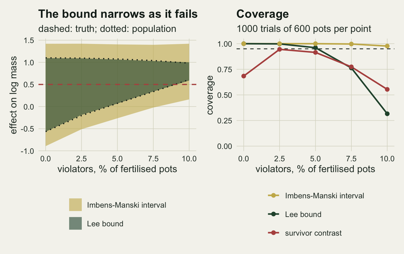

Figure 4: The bound when the fertiliser kills some seedlings that would have lived. Left: median bound, Imbens-Manski interval and the population bound against the share of fertilised pots killed. Right: coverage of the true effect over 1000 trials of 600 pots.

What to report

Report the survival rate in each arm and the survival gap before any harvest result, with the number of pots in each arm. The gap is the diagnostic that says whether the experiment can answer a question about growth at all, and it is the one number that needs no assumption. If the treatment truly leaves survival alone, the survivor contrast is the effect, but a sample never shows that, and a small observed gap is not a licence: with 600 pots a gap of 0.12 already takes the survivor interval down to 0.894 coverage. Put the Imbens-Manski interval beside it; near zero gap it costs only width.

Report the survivor contrast under its own name: the difference in mean mass between surviving fertilised and surviving control plants. Yield per surviving plant is a real agronomic quantity, and for a grower who will replant the failures it may be the quantity of interest. The fault measured above is in the label, not in the calculation. Calling it the effect of the fertiliser on growth is what fails, and it fails more with every pot added.

When the question is about growth, report the Lee bound with the trim share and how it was computed, and put an Imbens-Manski interval around it. State monotonicity as an assumption, with the reason it is believed for this treatment, and say what was seen in the dead pots. If the bound spans zero, say that the design cannot determine the direction of the growth effect. That is a finding about the experiment, and it is worth more than a significant survivor contrast with the wrong centre.

Before the next trial, the lesson is in the design. Harvesting the dead pots at the time they die, or measuring a size covariate on every pot early in the season, gives the analysis information about the plants that were lost, and a trial that expects heavy mortality in one arm can be grown under conditions that keep more of the controls alive.

Honest limits

The simulation gives every pot the same harvest effect. Then the effect among always-survivors, which is what the bound is about, equals the effect on all pots. With effects that vary between plants, and in particular with a fertiliser that helps weak plants more, the always-survivor effect is a different number from the average effect, and nothing in the data identifies the effect on pots that would have died in one arm.

Vigour is one latent variable that acts on survival and harvest with fixed loadings. The size of the bias and the width of the bound both depend on how strongly vigour drives the harvest, which is a design constant here. The bias is proportional to that loading, and the bound widens with it because the harvest distribution it trims spreads out. A trial where survival and growth depend on different traits has little bias, but the bound, which cannot know that, is still wide, since it trims whatever spread the harvest has. None of the coverage figures should be carried to another loading without rerunning the code.

The analytic standard error of the bound is Lee’s asymptotic formula, coded by hand, and it was checked only against the Monte Carlo spread of the endpoints in this design. It is close away from zero gap and too large at zero, where the estimated trim share is folded against its boundary. A bootstrap of the whole trimming procedure is the common alternative, and it was not run at this replication. The Imbens-Manski interval over-covers at zero gap for a reason that is structural rather than a coding choice, and the refinements in Stoye 2009 were not tried.

Only one kind of monotonicity failure was simulated: deaths among the weakest fertilised seedlings. A treatment that kills the most vigorous plants, for example by making lush growth more attractive to a pest, moves the bound the other way. The violation shares are chosen to show the direction and the speed of the failure, not to estimate any real fertiliser’s toxicity.

Finally, covariates were not used. Lee 2009 shows that trimming within strata of a baseline covariate that predicts survival narrows the bound, and a seedling height recorded at transplanting is exactly such a covariate. That would be the first improvement to try on real data.

References

Horowitz JL, Manski CF 2000 Journal of the American Statistical Association 95(449):77-84 (10.1080/01621459.2000.10473902)

Zhang JL, Rubin DB 2003 Journal of Educational and Behavioral Statistics 28(4):353-368 (10.3102/10769986028004353)

Imbens GW, Manski CF 2004 Econometrica 72(6):1845-1857 (10.1111/j.1468-0262.2004.00555.x)

Lee DS 2009 Review of Economic Studies 76(3):1071-1102 (10.1111/j.1467-937X.2009.00536.x)

Stoye J 2009 Econometrica 77(4):1299-1315 (10.3982/ECTA7347)

Related tutorials

• Non-compliance in field experiments
• Collider bias and selection
• Lost collar signals and informative censoring
• Checking a monitoring design