library(ggplot2)

te_pal <- list(forest = "#275139", green = "#2f8f63", sage = "#93a87f",
               clay = "#b5534e", gold = "#cda23f", line = "#dad9ca",
               ink = "#16241d", paper = "#f5f4ee")

theme_te <- function() {
  theme_minimal(base_size = 12) +
    theme(panel.grid.minor = element_blank(),
          panel.grid.major = element_line(colour = "#e7e6dc"),
          plot.background = element_rect(fill = "#f5f4ee", colour = NA),
          panel.background = element_rect(fill = "#f5f4ee", colour = NA),
          plot.title = element_text(face = "bold", colour = te_pal$ink),
          axis.title = element_text(colour = "#2c3a31"),
          axis.text = element_text(colour = "#2c3a31"))
}Interference between experimental plots
R
causal inference
experimental design
ecology tutorial
When treatment leaks between plots the estimated contrast shrinks while the standard error does not. A simulation measures the bias, the buffer cost and a fix.
A grassland experiment: one hundred and forty-four square plots on a regular grid, half of them fertilised, half left alone, and a biomass harvest at the end of the season. The analysis is a two-sample comparison and takes one line. The design is balanced, the randomisation was done properly, the residuals look fine, and the confidence interval is narrow. Everything about the output says the number can be trusted.
Nitrogen does not respect plot boundaries. Some of it moves downslope in the first heavy rain and arrives in a neighbouring plot that was supposed to be a control. Seed set on a fertilised plot lands two metres away. Grasshoppers that grew fat on the treated plot walk into the control and eat there. In a predator exclosure the prey that would have been eaten swim out and are counted somewhere else. None of this is exotic: it happens whenever the thing being manipulated can move and the plots are close enough together to be convenient to sample.
The statistical assumption this breaks has a name. Rubin called it the stable unit treatment value assumption, usually shortened to SUTVA, and it has two parts: there are no hidden versions of the treatment, and the outcome of a unit depends only on the treatment assigned to that unit rather than on the treatments assigned to any other unit. When the second part fails, the units are said to interfere with each other, and almost everything a standard analysis prints becomes a statement about a quantity nobody asked for.
Two nearby ideas need clearing out of the way, because they use overlapping words. The older ecological meaning of interference is interference competition, where each forager’s intake rate falls as neighbours crowd in around it; that appears in checking an ideal free analysis and is a biological process operating within one patch, not a property of a design. And spatial lag and spatial error models use the word spillover for the indirect effect in an autoregressive model, where the spilling is the quantity you want and reporting only the direct coefficient understates the ecology. Here the spilling is contamination: the same arithmetic that made the spatial multiplier interesting makes the experimental contrast wrong.
Interference is also not pseudoreplication, though the two get filed together because both involve plots being too close. Pseudoreplication is about the scale of the error term, measurements within a unit being treated as independent units so the standard error comes out too small; interference is about whose treatment affects whose outcome. The two are orthogonal, and a design can have every error term at the right scale and still be destroyed by leakage.
This post simulates a leaky grid experiment and measures six things: how large the bias gets, what happens to the standard error while that bias accumulates, which half of the leakage does the damage, what a buffer strip buys and what it costs, what clustering the treatments moves and what it does not remove, and whether putting the neighbourhood into the model recovers the effect.
A leak that conserves mass
The generating model has to be specific about what leaking means, because two mechanisms hide under the same word. The first is export: a treated plot loses part of what the treatment gave it, since the nitrogen that washes out is no longer in the plot it was applied to and the grasshopper that walks into the control is not eating in the treated one. The second is import: a plot receives whatever its neighbours exported, and that happens to control plots and treated plots alike.
Write \(Z_i\) for the treatment indicator of plot \(i\) and let a treated plot export a fraction \(\lambda\) of its treatment effect \(\tau\), split equally among its eight surrounding neighbours. The outcome is then
\[Y_i = \mu + \tau(1 - \lambda) Z_i + \frac{\tau\lambda}{8} \sum_{j \in N(i)} Z_j + \varepsilon_i\]
which conserves the total: adding up over the whole grid gives \(\tau\) per treated plot, exactly as it would with no leakage at all. That makes the question sharp. The treatment still does everything it did, the effect has only been redistributed, and the design has to find it.
Everything below runs on a torus, so the left edge of the grid wraps onto the right and the top onto the bottom. That is hygiene rather than realism: a real grid has plots on its outer boundary with fewer neighbours than the interior ones, and that boundary effect would mix into every measurement here.
shift_torus <- function(M, dr, dc) {
  nr <- nrow(M); nc <- ncol(M)
  M[((seq_len(nr) - 1 - dr) %% nr) + 1, ((seq_len(nc) - 1 - dc) %% nc) + 1]
}

ring_offsets <- function(r) {
  g <- expand.grid(dr = -r:r, dc = -r:r)
  as.matrix(g[pmax(abs(g$dr), abs(g$dc)) == r, ])
}

ring_sum <- function(M, r) {
  off <- ring_offsets(r)
  out <- matrix(0, nrow(M), ncol(M))
  for (k in seq_len(nrow(off))) out <- out + shift_torus(M, off[k, 1], off[k, 2])
  out
}

off1 <- ring_offsets(1)
off2 <- ring_offsets(2)

side <- 12
n_plot <- side^2
mu_base <- 5
tau <- 1
sigma <- 0.6
leak <- 0.35

sim_grid <- function(seed, leak, phi1 = 1) {
  set.seed(seed)
  z <- rep(0L, n_plot)
  z[sample.int(n_plot, n_plot / 2)] <- 1L
  Z <- matrix(z, side, side)
  s1 <- as.vector(ring_sum(Z, 1))
  s2 <- as.vector(ring_sum(Z, 2))
  imported <- tau * leak * (phi1 * s1 / nrow(off1) +
                              (1 - phi1) * s2 / nrow(off2))
  exported <- tau * leak * z
  noise <- rnorm(n_plot, 0, sigma)
  data.frame(z = z, s1 = s1, s2 = s2,
             exported = exported, imported = imported,
             y_leak = mu_base + tau * z - exported + imported + noise,
             y_clean = mu_base + tau * z + noise)
}

print(c(plots = n_plot, treated = n_plot / 2,
        ring1_neighbours = nrow(off1), ring2_neighbours = nrow(off2),
        true_effect = tau, leak_fraction = leak, residual_sd = sigma))
plots treated ring1_neighbours ring2_neighbours
144.00 72.00 8.00 16.00
true_effect leak_fraction residual_sd
1.00 0.35 0.60 The grid holds 144 plots with 72 of them treated, each plot has 8 first-ring neighbours and 16 second-ring neighbours, the true effect is 1 unit of biomass, the residual standard deviation is 0.6, and 35 per cent of each treated plot’s effect leaves the plot. That leak fraction is deliberately unremarkable: a third of applied nitrogen moving out of a small plot over a season is not an unusual figure in fertilisation work, and a third of the insects on a two-metre plot ending up elsewhere over a summer would surprise nobody. One dataset first, analysed the way the design says it should be analysed.
d1 <- sim_grid(20260802, leak)
fit_leak <- lm(y_leak ~ z, data = d1)
fit_clean <- lm(y_clean ~ z, data = d1)

print(round(summary(fit_leak)$coefficients, 4))
Estimate Std. Error t value Pr(>|t|)
(Intercept) 5.0761 0.0763 66.5378 0
z 0.7350 0.1079 6.8127 0print(round(summary(fit_clean)$coefficients, 4)) Estimate Std. Error t value Pr(>|t|)
(Intercept) 4.8987 0.0763 64.1652 0
z 1.0899 0.1080 10.0944 0print(round(c(
mean_treated = mean(d1$y_leak[d1$z == 1]),
mean_control = mean(d1$y_leak[d1$z == 0]),
contrast_leak = unname(coef(fit_leak)[2]),
contrast_clean = unname(coef(fit_clean)[2]),
resid_sd_leak = summary(fit_leak)$sigma,
resid_sd_clean = summary(fit_clean)$sigma,
shapiro_p = unname(shapiro.test(residuals(fit_leak))$p.value)), 4)) mean_treated mean_control contrast_leak contrast_clean resid_sd_leak
5.8111 5.0761 0.7350 1.0899 0.6473
resid_sd_clean shapiro_p
0.6478 0.7566 The leaky dataset returns a contrast of 0.735 against a truth of 1, with a standard error of 0.1079 and a p-value far below anything that would raise an eyebrow; the same plots without leakage give 1.0899. The residual standard deviation is 0.6473 in the leaky version against 0.6478 in the clean one, and the residuals pass a normality test at 0.7566. No diagnostic fires.
The bias arrives without a warning
One dataset proves nothing, so run two thousand of them. Each replicate redraws the assignment and the noise, fits the same one-line model to the leaky and the clean outcome, and stores the estimate, its standard error, and the average amount imported by each arm.
n_rep <- 2000
est_leak <- se_leak <- est_clean <- se_clean <- numeric(n_rep)
imp_treated <- imp_control <- numeric(n_rep)

for (r in seq_len(n_rep)) {
  d <- sim_grid(20260802 + r, leak)
  m_l <- lm(y_leak ~ z, data = d)
  m_c <- lm(y_clean ~ z, data = d)
  est_leak[r] <- coef(m_l)[2]
  se_leak[r] <- summary(m_l)$coefficients[2, 2]
  est_clean[r] <- coef(m_c)[2]
  se_clean[r] <- summary(m_c)$coefficients[2, 2]
  imp_treated[r] <- mean(d$imported[d$z == 1])
  imp_control[r] <- mean(d$imported[d$z == 0])
}

tcrit <- qt(0.975, n_plot - 2)
bias_meas <- mean(est_leak) - tau
att_pct <- 100 * (1 - mean(est_leak) / tau)
se_ratio <- mean(se_leak) / mean(se_clean)
sd_ratio <- sd(est_leak) / sd(est_clean)
cov_true <- mean(abs(est_leak - tau) < tcrit * se_leak)
cov_att <- mean(abs(est_leak - tau * (1 - leak)) < tcrit * se_leak)
cov_clean <- mean(abs(est_clean - tau) < tcrit * se_clean)

print(round(c(mean_est_clean = mean(est_clean), mean_est_leak = mean(est_leak),
              bias = bias_meas, attenuation_pct = att_pct), 4))
mean_est_clean mean_est_leak bias attenuation_pct
0.9990 0.6468 -0.3532 35.3221 print(round(c(mean_se_clean = mean(se_clean), mean_se_leak = mean(se_leak),
se_ratio = se_ratio, sd_est_clean = sd(est_clean),
sd_est_leak = sd(est_leak), sd_ratio = sd_ratio), 4))mean_se_clean mean_se_leak se_ratio sd_est_clean sd_est_leak
0.0998 0.1003 1.0050 0.0989 0.0997
sd_ratio
1.0076 print(round(c(coverage_clean = cov_clean, coverage_of_truth = cov_true,
coverage_of_attenuated = cov_att,
power_leak = mean(abs(est_leak / se_leak) > tcrit)), 4)) coverage_clean coverage_of_truth coverage_of_attenuated
0.9520 0.0600 0.9485
power_leak
1.0000 Over 2000 replicates the clean estimator averages 0.999 and the leaky one averages 0.6468, so the treatment contrast has lost 35.32 per cent of itself. That is the headline, and the second number is why it is dangerous: the mean standard error went from 0.0998 to 0.1003, a ratio of 1.005. The estimate moved by a third and the reported precision by 0.5 per cent.
The spread of the estimates says the same: standard deviation 0.0989 across replicates without leakage and 0.0997 with it, a ratio of 1.0076. Leakage is not adding variability. It moves the whole sampling distribution sideways and leaves its shape alone, which is the definition of bias and the one thing the residuals cannot see.
Coverage makes that concrete. The nominal 95 per cent interval contains the true effect in 95.2 per cent of clean replicates and in 6 per cent of leaky ones, while containing the attenuated value \(\tau(1 - \lambda) =\) 0.65 in 94.85 per cent of them. The interval is not broken; it is working perfectly, on a different quantity. Power is untouched in the sense that matters least, the null being rejected in 100 per cent of replicates. A study like this publishes a highly significant result with a tight interval around a number that is a third too small.
dens_df <- rbind(
  data.frame(est = est_clean, kind = "No leakage"),
  data.frame(est = est_leak, kind = "35 per cent leaks out"))
bar_df <- data.frame(
  kind = c("No leakage", "35 per cent leaks out"),
  centre = c(mean(est_clean), mean(est_leak)),
  half = tcrit * c(mean(se_clean), mean(se_leak)),
  yy = c(1.05, 0.55))

ggplot(dens_df, aes(est, colour = kind, fill = kind)) +
  geom_density(alpha = 0.25, linewidth = 0.7, adjust = 1.1) +
  geom_vline(xintercept = tau, linetype = "dashed",
             colour = te_pal$ink, linewidth = 0.5) +
  geom_errorbar(data = bar_df, inherit.aes = FALSE,
                aes(y = yy, xmin = centre - half, xmax = centre + half,
                    colour = kind),
                orientation = "y", width = 0.25, linewidth = 0.7,
                show.legend = FALSE) +
  scale_colour_manual(values = c("No leakage" = te_pal$forest,
                                 "35 per cent leaks out" = te_pal$clay)) +
  scale_fill_manual(values = c("No leakage" = te_pal$green,
                               "35 per cent leaks out" = te_pal$clay)) +
  labs(x = "Estimated treatment contrast",
       y = "Density",
       colour = NULL, fill = NULL,
       title = "The estimate moves, the interval does not widen") +
  theme_te() +
  theme(legend.position = "bottom",
        plot.margin = margin(8, 14, 8, 8))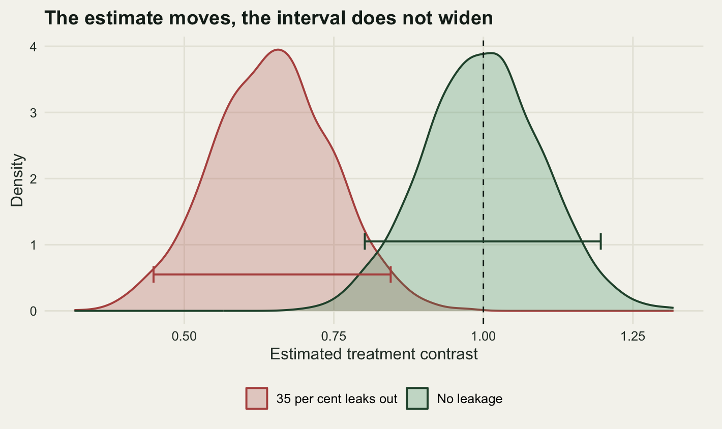
Which half of the leak does the damage
The intuition most people bring to this is that contaminating the controls is the problem: nitrogen arrives where it should not, the control plots grow more than they should, the gap closes. That intuition is half right, and the half it gets wrong changes what you would do about it.
The bias splits into three pieces. Treated plots lose \(\tau\lambda\) each through export; treated plots also gain whatever their own neighbours sent them; control plots gain the same way. Only the difference between the last two enters the contrast, and under an interspersed random assignment a treated plot has almost exactly as many treated neighbours as a control plot does.
export_loss <- tau * leak
import_t <- mean(imp_treated)
import_c <- mean(imp_control)
import_gap <- import_c - import_t
import_gap_se <- sd(imp_control - imp_treated) / sqrt(n_rep)
gap_pred <- tau * leak / (n_plot - 1)
bias_pred <- -(export_loss + gap_pred)

print(round(c(mean_import_treated = import_t,
              mean_import_control = import_c,
              import_gap = import_gap,
              import_gap_mc_se = import_gap_se,
              import_gap_predicted = gap_pred), 6))
mean_import_treated mean_import_control import_gap
0.173892 0.176108 0.002217
import_gap_mc_se import_gap_predicted
0.000324 0.002448 print(round(c(export_component = -export_loss,
control_contamination_component = -import_gap,
predicted_total_bias = bias_pred,
measured_total_bias = bias_meas), 5)) export_component control_contamination_component
-0.35000 -0.00222
predicted_total_bias measured_total_bias
-0.35245 -0.35322 print(round(c(export_share_pct = 100 * export_loss / abs(bias_pred),
contamination_share_pct = 100 * gap_pred / abs(bias_pred)), 3)) export_share_pct contamination_share_pct
99.306 0.694 Control plots do get contaminated, by an average of 0.1761 units of biomass, 17.61 per cent of the effect being chased. If that were the whole story the contrast would fall by that much. But treated plots are contaminated by 0.1739 units, almost the same, and only the gap of 0.002217 survives into the contrast.
That gap is not zero, and its size is predictable. Under a completely randomised assignment of 72 treated plots out of 144, a control plot’s neighbour is treated with probability \(m/(n-1)\) and a treated plot’s neighbour with probability \((m-1)/(n-1)\), so the expected difference in imports is exactly \(\tau\lambda/(n-1) =\) 0.002448. The measured value over 2000 replicates is 0.002217, with a Monte Carlo standard error of 0.000324.
The accounting comes out at 99.31 per cent export and 0.69 per cent control contamination, with a predicted total bias of -0.35245 against the measured -0.35322. This went against what I expected before running it. Contaminated controls are the part everyone worries about, and in a well-interspersed design they are almost entirely self-cancelling, because the treated plots are contaminated at the same rate by each other. What survives is the export: the treated plots do not show the whole effect, because part of it is no longer there.
That has a design consequence. If the treatment depletes the source when it spreads, which covers leaching, seed dispersal and animal movement, then shielding the controls fixes almost nothing on its own; what has to be protected is the treated plot’s own budget. If it does not deplete the source, a light or temperature manipulation whose halo does not dim the centre, the same arithmetic says the interspersed contrast is nearly unbiased for the direct effect, both arms taking on the same halo. Which of the two you are in is a question about the mechanism, and no amount of looking at the data will settle it.
Buffers, and what the sample size costs
The standard field answer to leakage is a buffer: make each plot bigger than the area you sample and take the measurements from the middle. If leakage reaches a fixed distance into the plot and the buffer is at least as wide as that, the sampled part never sees the neighbour’s treatment at all.
Modelling that needs a finer grain than one value per plot. Take 64 plots, each divided into a 9-by-9 array of quadrats, and let the treatment effect at a quadrat be the average treatment over a disc of fixed radius around it. A quadrat in the middle of a treated plot has a disc lying entirely inside the plot and gets the full effect; a quadrat on the plot edge has part of its disc in a neighbour and gets a diluted version. In field terms: a 4.5 metre plot in 0.5 metre quadrats, with material moving up to one metre.
disc_offsets <- function(r) {
  g <- expand.grid(dr = -r:r, dc = -r:r)
  as.matrix(g[g$dr^2 + g$dc^2 <= r^2, ])
}

disc_mean <- function(M, off) {
  out <- matrix(0, nrow(M), ncol(M))
  for (k in seq_len(nrow(off))) out <- out + shift_torus(M, off[k, 1], off[k, 2])
  out / nrow(off)
}

p_side <- 8
k_sub <- 9
rho <- 2
np2 <- p_side^2
g_side <- p_side * k_sub
off_disc <- disc_offsets(rho)

sub_row <- rep(seq_len(g_side), times = g_side)
sub_col <- rep(seq_len(g_side), each = g_side)
plot_id <- ((sub_col - 1) %/% k_sub) * p_side + (sub_row - 1) %/% k_sub + 1
in_r <- (sub_row - 1) %% k_sub
in_c <- (sub_col - 1) %% k_sub
depth <- pmin(in_r, k_sub - 1 - in_r, in_c, k_sub - 1 - in_c)

sigma_u <- 0.15
buffers <- 0:3
keep_list <- lapply(buffers, function(b) depth >= b)
n_kept <- sapply(keep_list, function(k) sum(k) / np2)

print(c(plots = np2, quadrats_per_plot = k_sub^2, disc_cells = nrow(off_disc),
        interference_radius = rho, plot_sd = sigma_u))
plots quadrats_per_plot disc_cells interference_radius
64.00 81.00 13.00 2.00
plot_sd
0.15 print(rbind(buffer = buffers, quadrats_kept = n_kept)) [,1] [,2] [,3] [,4]
buffer 0 1 2 3
quadrats_kept 81 49 25 9There are 64 plots of 81 quadrats each, the interference disc covers 13 quadrats out to a radius of 2, and the buffer widths under test drop the retained sample per plot from 81 quadrats to 9. Because the treatment is assigned at plot level, the analysis has to be at plot level too: average the retained quadrats within each plot, then compare the 32 treated plot means with the 32 control ones. Doing anything else would be the pseudoreplication error, and it would hide the buffer’s cost rather than reveal it. That cost depends on how noisy the quadrats are relative to the plots, so the sweep runs at five levels of quadrat noise with the plot-level standard deviation held fixed.
sig_e_grid <- c(1.2, 2, 3, 4, 5)
n_rep_b <- 500
nb <- length(buffers)
ns <- length(sig_e_grid)
acc_e <- acc_e2 <- acc_se <- acc_cov <- matrix(0, nb, ns)

for (r in seq_len(n_rep_b)) {
  set.seed(31000 + r)
  zp <- rep(0L, np2)
  zp[sample.int(np2, np2 / 2)] <- 1L
  Zp <- matrix(zp, p_side, p_side)
  Zsub <- Zp[rep(seq_len(p_side), each = k_sub),
             rep(seq_len(p_side), each = k_sub)]
  expo <- as.vector(disc_mean(Zsub, off_disc))
  u_p <- rnorm(np2, 0, sigma_u)[plot_id]
  e_raw <- rnorm(g_side^2)
  base <- mu_base + tau * expo + u_p
  for (js in seq_len(ns)) {
    yv <- base + sig_e_grid[js] * e_raw
    for (jb in seq_len(nb)) {
      kk <- keep_list[[jb]]
      pm <- as.vector(tapply(yv[kk], plot_id[kk], mean))
      mf <- lm(pm ~ zp)
      dd <- unname(coef(mf)[2])
      ss <- summary(mf)$coefficients[2, 2]
      acc_e[jb, js] <- acc_e[jb, js] + dd
      acc_e2[jb, js] <- acc_e2[jb, js] + dd^2
      acc_se[jb, js] <- acc_se[jb, js] + ss
      acc_cov[jb, js] <- acc_cov[jb, js] + (abs(dd - tau) < qt(0.975, np2 - 2) * ss)
    }
  }
}

buf <- expand.grid(buffer = buffers, sigma_e = sig_e_grid)
buf$mean_est <- as.vector(acc_e) / n_rep_b
buf$variance <- as.vector(acc_e2) / n_rep_b - buf$mean_est^2
buf$mean_se <- as.vector(acc_se) / n_rep_b
buf$coverage <- as.vector(acc_cov) / n_rep_b
buf$bias <- buf$mean_est - tau
buf$bias2 <- buf$bias^2
buf$mse <- buf$bias2 + buf$variance
buf$kept <- n_kept[buf$buffer + 1]
qq <- function(b, s, col) buf[[col]][buf$buffer == b & buf$sigma_e == s]

print(round(buf[buf$sigma_e %in% c(1.2, 3, 5),
                c("buffer", "sigma_e", "kept", "mean_est", "bias",
                  "variance", "mse", "coverage")], 5))
buffer sigma_e kept mean_est bias variance mse coverage
1 0 1.2 81 0.83095 -0.16905 0.00251 0.03109 0.088
2 1 1.2 49 0.95603 -0.04397 0.00329 0.00523 0.882
3 2 1.2 25 1.00004 0.00004 0.00485 0.00485 0.956
4 3 1.2 9 1.00093 0.00093 0.01160 0.01160 0.940
9 0 3.0 81 0.83244 -0.16756 0.00766 0.03573 0.538
10 1 3.0 49 0.95768 -0.04232 0.01275 0.01454 0.946
11 2 3.0 25 1.00081 0.00081 0.02276 0.02276 0.956
12 3 3.0 9 1.00303 0.00303 0.06351 0.06352 0.946
17 0 5.0 81 0.83410 -0.16590 0.01863 0.04615 0.814
18 1 5.0 49 0.95951 -0.04049 0.03258 0.03422 0.944
19 2 5.0 25 1.00167 0.00167 0.06058 0.06059 0.952
20 3 5.0 9 1.00536 0.00536 0.17272 0.17275 0.942best <- tapply(seq_len(nrow(buf)), buf$sigma_e,
function(i) buf$buffer[i][which.min(buf$mse[i])])
print(rbind(sigma_e = sig_e_grid, best_buffer = as.vector(best))) [,1] [,2] [,3] [,4] [,5]
sigma_e 1.2 2 3 4 5
best_buffer 2.0 1 1 1 1With no buffer the estimate averages 0.8309 against a truth of 1, a 16.91 per cent attenuation, and at the lowest noise level the nominal interval covers the truth 8.8 per cent of the time. Discarding one ring of quadrats cuts the bias to -0.044. Discarding two rings, the true interference radius, leaves 0.00004 and brings coverage back to 95.6 per cent.
The price is in the third column. Going from no buffer to two rings throws away 69.14 per cent of the quadrats, and the variance of the plot-level contrast rises from 0.00251 to 0.00485. At this noise level that is still worth paying, but only just: the mean squared error is 0.00523 at one ring and 0.00485 at two, a gap of 7.78 per cent. That margin is where the design decision lives, and it flips.
b1 <- buf[buf$buffer == 1, ]
b2 <- buf[buf$buffer == 2, ]
n_arm <- np2 / 2
kept1 <- n_kept[2]
kept2 <- n_kept[3]

bias2_gain <- mean(b1$bias)^2 - mean(b2$bias)^2
var_slope <- (2 / n_arm) * (1 / kept1 - 1 / kept2)
sigma_star <- sqrt(bias2_gain / (-var_slope))

fit_v1 <- lm(b1$variance ~ I(sig_e_grid^2))
fit_v2 <- lm(b2$variance ~ I(sig_e_grid^2))

print(round(c(mean_bias_buffer1 = mean(b1$bias),
              mean_bias_buffer2 = mean(b2$bias),
              squared_bias_gain = bias2_gain,
              variance_slope_per_sigma2 = var_slope,
              break_even_sigma_e = sigma_star), 5))
mean_bias_buffer1 mean_bias_buffer2 squared_bias_gain
-0.04228 0.00083 0.00179
variance_slope_per_sigma2 break_even_sigma_e
-0.00122 1.20813 print(round(c(fitted_slope_buffer1 = unname(coef(fit_v1)[2]),
predicted_slope_buffer1 = (2 / n_arm) / kept1,
fitted_slope_buffer2 = unname(coef(fit_v2)[2]),
predicted_slope_buffer2 = (2 / n_arm) / kept2), 5)) fitted_slope_buffer1 predicted_slope_buffer1 fitted_slope_buffer2
0.00124 0.00128 0.00237
predicted_slope_buffer2
0.00250 print(round(buf$mse[buf$buffer == 1] - buf$mse[buf$buffer == 2], 5))[1] 0.00038 -0.00254 -0.00822 -0.01616 -0.02636The variance of a plot-level contrast is \((2/m)(\sigma_u^2 + \sigma_e^2/q)\) for \(m\) plots per arm and \(q\) quadrats retained per plot, so widening the buffer by one ring raises it by an amount proportional to \(\sigma_e^2\), while the squared bias it removes is a fixed quantity. Setting the two equal gives a break-even quadrat noise of 1.2081. Below that, buffer to the full interference radius; above it, the wider buffer costs more variance than the bias is worth, and the MSE-optimal buffer is one ring, narrower than the true interference range, deliberately leaving a bias of -0.0423 on the table.
The fitted variance slopes confirm the arithmetic: 0.00124 against a predicted 0.00128 at one ring, and 0.00237 against 0.0025 at two. The sweep over the five noise levels puts the optimum at 2 rings for the quietest quadrats and 1 ring for the noisiest, crossing where the formula says it should.
Two further readings of that table. Buffering past the interference radius is never right: at three rings the bias is already gone and the MSE is 2.392 times the two-ring value at the lowest noise. And the unbuffered coverage improves as the quadrats get noisier, from 8.8 to 81.4 per cent, which is not good news: the estimate is just as wrong, and the interval has simply grown wide enough to cover the truth by accident.
plot_lv <- c(1.2, 3, 5)
bf <- buf[buf$sigma_e %in% plot_lv, ]
bf$panel <- factor(paste("Quadrat noise", bf$sigma_e),
                   levels = paste("Quadrat noise", plot_lv))
parts <- c("Squared bias", "Variance", "Mean squared error")
long <- do.call(rbind, Map(function(v, p)
  data.frame(buffer = bf$buffer, panel = bf$panel, value = v, part = p),
  list(bf$bias2, bf$variance, bf$mse), parts))
long$part <- factor(long$part, levels = parts)
mins <- do.call(rbind, lapply(split(bf, bf$panel), function(s)
  s[which.min(s$mse), c("buffer", "mse", "panel")]))

ggplot(long, aes(buffer, value, colour = part)) +
  geom_line(linewidth = 0.75) +
  geom_point(size = 1.6) +
  geom_point(data = mins, inherit.aes = FALSE,
             aes(buffer, mse), shape = 21, size = 4.2, stroke = 1,
             colour = te_pal$ink, fill = NA) +
  facet_wrap(~panel, scales = "free_y") +
  scale_colour_manual(values = c("Squared bias" = te_pal$clay,
                                 "Variance" = te_pal$gold,
                                 "Mean squared error" = te_pal$forest)) +
  labs(x = "Buffer width (rings of quadrats discarded)",
       y = "Contribution to error",
       colour = NULL,
       title = "Where the buffer stops paying for itself") +
  theme_te() +
  theme(legend.position = "bottom",
        plot.margin = margin(8, 14, 8, 8))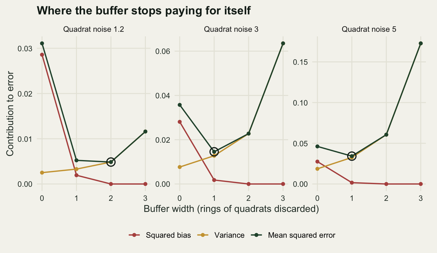
Layout moves the failure rather than removing it
If contamination between arms is the mechanism, then putting the treated plots together and the control plots together should reduce it, because most of a treated plot’s neighbours would then be treated as well. That is true, and it is a real design lever. It is also a trade rather than a fix.
The comparison holds the leak fraction fixed and changes only the assignment. In the interspersed layout, 72 of the 144 plots are treated at random; in the clustered layout, the grid is cut into three-by-three blocks and half the blocks are treated whole, so a treated plot usually has treated neighbours. To make the cost visible, the site now carries a smooth environmental field, generated by smoothing white noise over a five-plot window, of the kind that soil depth or drainage produces at any real site.
box_smooth <- function(M, r) {
  out <- matrix(0, nrow(M), ncol(M))
  for (dr in -r:r) for (dc in -r:r) out <- out + shift_torus(M, dr, dc)
  out / (2 * r + 1)^2
}

blk <- 3
n_blk <- (side / blk)^2
field_sd <- 0.5

run_layout <- function(mode, n_rep_l = 2000, seed0 = 47000) {
  est <- se <- imp_t <- imp_c <- fld <- numeric(n_rep_l)
  for (r in seq_len(n_rep_l)) {
    set.seed(seed0 + r)
    if (mode == "interspersed") {
      z <- rep(0L, n_plot)
      z[sample.int(n_plot, n_plot / 2)] <- 1L
      Z <- matrix(z, side, side)
    } else {
      bm <- matrix(0L, side / blk, side / blk)
      bm[sample.int(n_blk, n_blk / 2)] <- 1L
      Z <- bm[rep(seq_len(side / blk), each = blk),
              rep(seq_len(side / blk), each = blk)]
      z <- as.vector(Z)
    }
    imported <- tau * leak * as.vector(ring_sum(Z, 1)) / nrow(off1)
    fv <- as.vector(scale(as.vector(
      box_smooth(matrix(rnorm(n_plot), side, side), 2)))) * field_sd
    y <- mu_base + tau * z - tau * leak * z + imported + fv +
      rnorm(n_plot, 0, sigma)
    mf <- lm(y ~ z)
    est[r] <- coef(mf)[2]
    se[r] <- summary(mf)$coefficients[2, 2]
    imp_t[r] <- mean(imported[z == 1])
    imp_c[r] <- mean(imported[z == 0])
    fld[r] <- mean(fv[z == 1]) - mean(fv[z == 0])
  }
  data.frame(est = est, se = se, imp_t = imp_t, imp_c = imp_c, fld = fld)
}

lay_int <- run_layout("interspersed")
lay_clu <- run_layout("clustered")

lay_row <- function(x, nm) data.frame(
  layout = nm, mean_est = mean(x$est), bias = mean(x$est) - tau,
  sd_est = sd(x$est), mean_se = mean(x$se),
  import_gap = mean(x$imp_t - x$imp_c), field_gap_sd = sd(x$fld),
  coverage = mean(abs(x$est - tau) < tcrit * x$se),
  rmse = sqrt(mean((x$est - tau)^2)))
lay_tab <- rbind(lay_row(lay_int, "interspersed"),
                 lay_row(lay_clu, "clustered"))
lay_tab$se_honesty <- lay_tab$sd_est / lay_tab$mean_se
print(round(lay_tab[, -1], 5))
mean_est bias sd_est mean_se import_gap field_gap_sd coverage rmse
1 0.65108 -0.34892 0.12617 0.13076 -0.00231 0.08223 0.2375 0.37102
2 0.82923 -0.17077 0.22028 0.12995 0.18351 0.19648 0.6145 0.27867
se_honesty
1 0.96486
2 1.69506print(lay_tab$layout)[1] "interspersed" "clustered" Clustering does what it promises. The attenuation falls from 34.89 per cent to 17.08 per cent, roughly halved, because the import gap between the arms, treated minus control, goes from -0.0023 to 0.1835: treated plots are now contaminated by their treated neighbours far more than control plots are, and that gap pushes the contrast back towards the truth.
The bill arrives in the spread columns. The standard deviation of the estimate across randomisations goes from 0.1262 under interspersion to 0.2203 under clustering, while the standard error the model reports barely moves, 0.1308 against 0.13. The ratio of the two, which should be one, is 0.965 interspersed and 1.695 clustered. The environmental field is the reason: the difference in field means between the arms has a standard deviation of 0.0822 when plots are interspersed and 0.1965 when they are clumped, since a clumped assignment can land the whole treated group on the wetter half of the site.
Root mean squared error prefers the clustered design here, 0.2787 against 0.371, and coverage is better too, 61.45 per cent against 23.75 per cent. Neither is close to 95. What clustering has done is convert a bias, stable and open to reasoning and partial correction, into a randomisation variance that the reported standard error understates by a factor of 1.695. Two clustered studies can disagree sharply and both report tight intervals. The choice is between two ways of being wrong, and the clustered one is harder to detect after the fact.
lay_df <- rbind(
  data.frame(est = lay_int$est, layout = "Interspersed"),
  data.frame(est = lay_clu$est, layout = "Clustered blocks"))
lay_mean <- data.frame(
  layout = c("Interspersed", "Clustered blocks"),
  m = c(mean(lay_int$est), mean(lay_clu$est)))

ggplot(lay_df, aes(est, colour = layout, fill = layout)) +
  geom_density(alpha = 0.22, linewidth = 0.7, adjust = 1.1) +
  geom_vline(xintercept = tau, linetype = "dashed",
             colour = te_pal$ink, linewidth = 0.5) +
  geom_rug(data = lay_mean, inherit.aes = FALSE,
           aes(x = m, colour = layout), linewidth = 1.1,
           length = unit(0.05, "npc"), show.legend = FALSE) +
  scale_colour_manual(values = c("Interspersed" = te_pal$clay,
                                 "Clustered blocks" = te_pal$forest)) +
  scale_fill_manual(values = c("Interspersed" = te_pal$clay,
                               "Clustered blocks" = te_pal$green)) +
  labs(x = "Estimated treatment contrast",
       y = "Density", colour = NULL, fill = NULL,
       title = "Clustering trades bias for randomisation variance") +
  theme_te() +
  theme(legend.position = "bottom",
        plot.margin = margin(8, 14, 8, 8))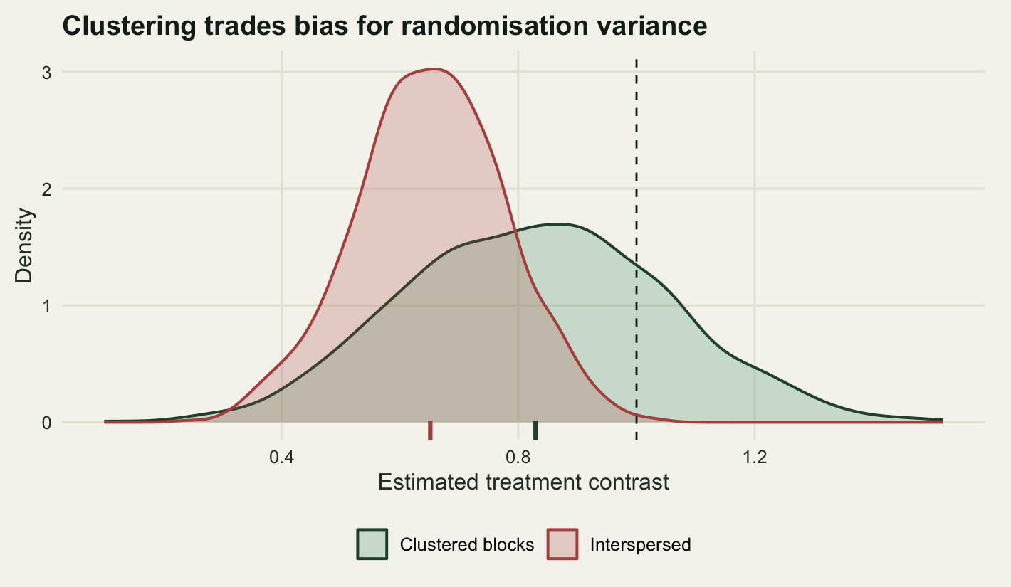
Putting the neighbours in the model
If the neighbourhood of every plot was recorded, and on a grid it always is, then the number of treated neighbours is a variable like any other and can go into the regression. Fitting
\[Y_i = \alpha + \beta Z_i + \gamma S_i + \varepsilon_i\]
with \(S_i\) the count of treated first-ring neighbours is a correctly specified model for the generating process used above. The question is what to read off it. The coefficient \(\beta\) is the direct effect of treating a plot on that plot, which under export is \(\tau(1 - \lambda)\) and still understates the treatment; the full effect of treating one plot, counting what it does to its eight neighbours, is \(\beta + 8\gamma\), and that is what compares against \(\tau\).
combo <- function(fit, wts) {
  b <- coef(fit)
  kv <- setNames(rep(0, length(b)), names(b))
  kv[names(wts)] <- unlist(wts)
  c(est = sum(kv * b), se = sqrt(drop(t(kv) %*% vcov(fit) %*% kv)))
}

run_cov <- function(phi1, n_rep_c = 1500, seed0 = 61000) {
  out <- matrix(NA_real_, n_rep_c, 9)
  for (r in seq_len(n_rep_c)) {
    d <- sim_grid(seed0 + r, leak, phi1)
    m0 <- lm(y_leak ~ z, data = d)
    m1 <- lm(y_leak ~ z + s1, data = d)
    m2 <- lm(y_leak ~ z + s1 + s2, data = d)
    out[r, ] <- c(combo(m0, list(z = 1)),
                  combo(m1, list(z = 1, s1 = nrow(off1))),
                  combo(m2, list(z = 1, s1 = nrow(off1), s2 = nrow(off2))),
                  unname(coef(m1)["z"]), unname(coef(m1)["s1"]),
                  cor(d$s1, d$s2))
  }
  colnames(out) <- c("e0", "s0", "e1", "s1", "e2", "s2",
                     "direct1", "gamma1", "cor12")
  as.data.frame(out)
}

cov_near <- run_cov(1)
cov_far <- run_cov(0.7)

summ_cov <- function(x, label) data.frame(
  truth = label,
  model = c("treatment only", "plus ring 1", "plus rings 1 and 2"),
  est = c(mean(x$e0), mean(x$e1), mean(x$e2)),
  se = c(mean(x$s0), mean(x$s1), mean(x$s2)),
  cover = c(mean(abs(x$e0 - tau) < tcrit * x$s0),
            mean(abs(x$e1 - tau) < tcrit * x$s1),
            mean(abs(x$e2 - tau) < tcrit * x$s2)))
rec <- rbind(summ_cov(cov_near, "all leakage in ring 1"),
             summ_cov(cov_far, "70 per cent ring 1, 30 per cent ring 2"))
rec$recovered_pct <- 100 * rec$est / tau
print(round(rec[, c("est", "se", "cover", "recovered_pct")], 4))
est se cover recovered_pct
1 0.6467 0.1005 0.0700 64.6689
2 0.9909 0.3155 0.9400 99.0895
3 1.0045 0.5837 0.9560 100.4529
4 0.6467 0.1003 0.0700 64.6700
5 0.8765 0.3156 0.9293 87.6521
6 1.0045 0.5837 0.9560 100.4529print(rec[, c("truth", "model")]) truth model
1 all leakage in ring 1 treatment only
2 all leakage in ring 1 plus ring 1
3 all leakage in ring 1 plus rings 1 and 2
4 70 per cent ring 1, 30 per cent ring 2 treatment only
5 70 per cent ring 1, 30 per cent ring 2 plus ring 1
6 70 per cent ring 1, 30 per cent ring 2 plus rings 1 and 2print(round(c(direct_coef_ring1_model = mean(cov_near$direct1),
attenuated_truth = tau * (1 - leak),
se_inflation_ring1 = rec$se[2] / rec$se[1],
se_inflation_ring12 = rec$se[3] / rec$se[1]), 4))direct_coef_ring1_model attenuated_truth se_inflation_ring1
0.6494 0.6500 3.1390
se_inflation_ring12
5.8073 When the assumed range is right, the model works. With all leakage confined to the first ring, the treatment-only estimate recovers 64.67 per cent of the effect and the ring-1 model recovers 99.09 per cent, with coverage of 94 per cent against 7 per cent. The direct coefficient there averages 0.6494, which is \(\tau(1 - \lambda) =\) 0.65 and not the answer; the answer appears only once the eight neighbour terms are added back.
The cost is precision. The standard error on the total effect is 0.3155 under the ring-1 model against 0.1005 for the naive contrast, an inflation of 3.139 times, and adding the second ring when it is not needed takes it to 0.5837, or 5.807 times the naive value. That is the exchange rate: the biased estimator was precise about the wrong quantity, and the unbiased one buys the right quantity at a threefold wider interval.
Now the part that decides whether this is usable. The second block of rows has the same total leakage, but 30 per cent of it reaches the second ring instead of the first, and the analyst fitting the ring-1 model does not know that.
short_recovery <- rec$recovered_pct[5]
full_recovery <- rec$recovered_pct[6]
shortfall <- rec$est[2] - rec$est[5]
beyond <- tau * leak * 0.3
print(round(c(ring1_model_wrong_range = rec$est[5],
              ring1_model_right_range = rec$est[2],
              full_model_either_truth = rec$est[6],
              recovery_pct_wrong_range = short_recovery,
              shortfall = shortfall,
              leakage_beyond_assumed_range = beyond,
              overshoot = shortfall - beyond), 4))
ring1_model_wrong_range ring1_model_right_range
0.8765 0.9909
full_model_either_truth recovery_pct_wrong_range
1.0045 87.6521
shortfall leakage_beyond_assumed_range
0.1144 0.1050
overshoot
0.0094 print(round(c(coverage_wrong_range = rec$cover[5],
coverage_right_range = rec$cover[2],
bias_in_se_units = (tau - rec$est[5]) / rec$se[5]), 4))coverage_wrong_range coverage_right_range bias_in_se_units
0.9293 0.9400 0.3913 print(round(c(gamma1_right_range = mean(cov_near$gamma1),
gamma1_wrong_range = mean(cov_far$gamma1),
gamma1_if_no_absorption = tau * leak * 0.7 / nrow(off1),
mean_cor_s1_s2 = mean(cov_far$cor12)), 5)) gamma1_right_range gamma1_wrong_range gamma1_if_no_absorption
0.04269 0.02854 0.03062
mean_cor_s1_s2
-0.11017 Assuming a range that is too short recovers 87.65 per cent of the effect instead of 100.45. The shortfall against the correctly specified version of the same model is 0.1144, a little more than the 0.105 that actually went past the assumed range. The extra 0.0094 comes from the omitted second ring dragging the first-ring coefficient down with it, 0.02854 against the 0.03062 that ring-1 leakage alone would give, the two neighbour counts carrying a small negative correlation of -0.11017 under a completely randomised assignment.
Coverage barely reacts: 92.93 per cent with the wrong range against 94 with the right one. That is not reassurance. The bias is 0.391 standard errors, and an interval that had to grow 3.139 times wider to be unbiased in the first place is wide enough to swallow a mistake of that size without registering it.
One exact property is hiding in those numbers. The full model returns 1.0045 under both truths, to the last digit printed: the two outcome vectors differ by a quantity lying exactly in the span of the two neighbour counts, and the contrast \(\beta + 8\gamma_1 + 16\gamma_2\) is built to absorb the whole of that span. Once the assumed range covers the true range, how the leakage is distributed inside it stops mattering. That is also the trap, because nothing in the fitting process says where the true range ends. The mismatched ring-1 model has an ordinary summary and residuals that give no sign of the ring-2 term left out of it.
rec$model <- factor(rec$model, levels = rev(unique(rec$model)))
rec$truth <- factor(rec$truth, levels = unique(rec$truth))
rec$lo <- rec$est - tcrit * rec$se
rec$hi <- rec$est + tcrit * rec$se

ggplot(rec, aes(est, model)) +
  geom_vline(xintercept = tau, linetype = "dashed",
             colour = te_pal$ink, linewidth = 0.5) +
  geom_errorbar(aes(xmin = lo, xmax = hi), orientation = "y", width = 0.18,
                colour = te_pal$sage, linewidth = 0.8) +
  geom_point(size = 3, colour = te_pal$forest) +
  scale_x_continuous(expand = expansion(mult = 0.07)) +
  facet_wrap(~truth, ncol = 1) +
  labs(x = "Recovered total effect of treating one plot",
       y = NULL,
       title = "The covariate fix works only out to the assumed range") +
  theme_te() +
  theme(plot.margin = margin(8, 18, 8, 8))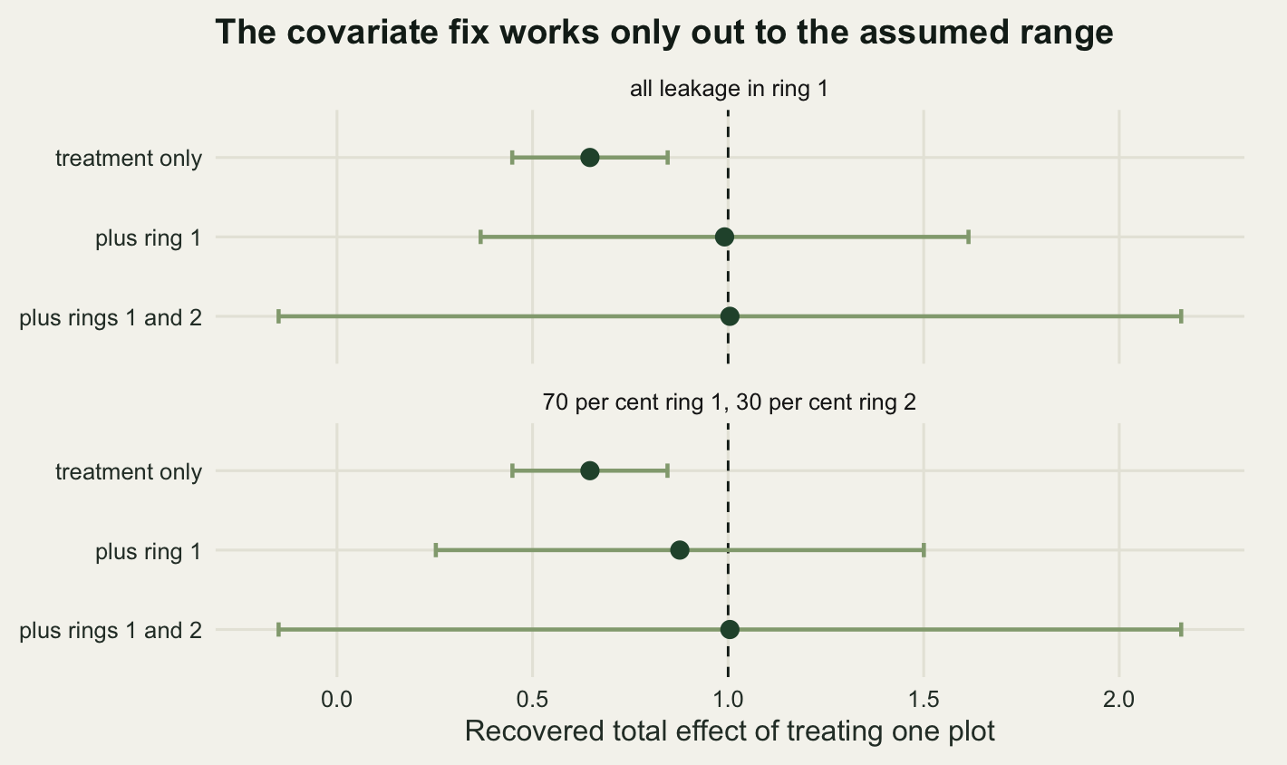
What to take away
Leakage between plots is a bias, not extra noise, and that single fact explains why it survives peer review so easily. In the base simulation it removed 35.32 per cent of the treatment contrast while changing the standard error by 0.5 per cent and the spread of the estimates by 0.76 per cent. The nominal interval covered the truth 6 per cent of the time and the attenuated quantity 94.85 per cent of the time: a working interval pointed at the wrong target. No residual plot and no measure of precision has any purchase on that, because nothing about the fitted model is malfunctioning.
Two measurements went against the intuition I started with. Contaminated controls, the part that gets the attention, contributed 0.69 per cent of the bias, because in an interspersed design the treated plots are contaminated at almost exactly the same rate and the two cancel; export from the treated plots contributed the other 99.31 per cent. And the buffer that minimises mean squared error is not always the buffer that removes the bias: past a quadrat noise of 1.2081 it pays to keep a ring known to be contaminated, carrying a bias of -0.0423 in exchange for the sample size.
Every design lever cost something measurable. A buffer to the full interference radius threw away 69.14 per cent of the quadrats; clustering the treatments halved the bias and inflated the true spread of the estimate to 1.695 times the standard error the model reported; putting the neighbour count in the model recovered the full effect but multiplied the standard error by 3.139, or 5.807 with a second ring added as insurance.
The honest limit is the interference range. Every correction here worked because the simulation was told how far the leakage reached, and when it was told wrong by one ring the covariate model recovered 87.65 per cent instead of 100.45 per cent while its coverage held at 92.93 per cent, the interval by then being wide enough to hide a bias of 0.391 standard errors. Reading the range off the same experiment is not a way out: fitting one extra ring as insurance already cost a factor of 1.85 in the standard error of the answer, so a model carrying enough rings to discover the range has no precision left to report. The number has to come from the mechanism, from a tracer study or a mark-recapture estimate of movement distance, and it has to be settled before the plots are laid out, because by the time the biomass is in the bags the spacing is fixed and the only remaining choice is which quadrats to discard.
References
Rubin DB 1980 Journal of the American Statistical Association 75(371):591-593 (10.1080/01621459.1980.10477517)
Hudgens MG, Halloran ME 2008 Journal of the American Statistical Association 103(482):832-842 (10.1198/016214508000000292)
Sobel ME 2006 Journal of the American Statistical Association 101(476):1398-1407 (10.1198/016214506000000636)
Aronow PM, Samii C 2017 Annals of Applied Statistics 11(4):1912-1947 (10.1214/16-AOAS1005)
Baird S, Bohren JA, McIntosh C, Ozler B 2018 The Review of Economics and Statistics 100(5):844-860 (10.1162/rest_a_00716)
Englund G 1997 Ecology 78(8):2316-2325 (10.2307/2265894)
Hurlbert SH 1984 Ecological Monographs 54(2):187-211 (10.2307/1942661)