---
title: "Checking an ideal free analysis"
description: "Three checks for an ideal free distribution study in R: is fitness really equalised, are competitors equal, and why the matching slope cannot name a mechanism."
date: "2026-07-03 11:00"
date-modified: "2026-10-15"
categories: [ecology tutorial, R, habitat selection, model diagnostics, behaviour]
image: thumbnail.png
image-alt: "Fitness across individuals equalised under an ideal free distribution but unequal under a despotic one, with dominants doing better."
---
*Corrected 15 October 2026: the post said that a departure of the matching slope shows that some ideal free assumption is relaxed, that a large coefficient of variation in intake points to despotism, and that higher fitness in the good habitat means the animals are not distributing freely; it now says that strong interference alone gives undermatching with the same intake in every patch, that competitors of unequal ability who exclude no one also give a large coefficient of variation, and that higher fitness in the good habitat shows only that the animals are not at an ideal free distribution.*
*Corrected 7 October 2026: the post said that a despotic distribution can reproduce input matching in the counts while producing unequal payoffs; under its own rule that each patch's input is shared equally among the animals in it, matched counts give everyone the same intake, so the sentence now says this also needs dominants to take a larger share within a patch.*
```{r setup}
#| code-fold: true
#| code-summary: "Setup: packages, colours and plot theme"
#| results: hide
#| message: false
#| warning: false
knitr::opts_chunk$set(echo = TRUE, message = FALSE, warning = FALSE,
                      dev = "png", dpi = 120, fig.path = "figures/",
                      fig.width = 7, fig.height = 4.4)
library(ggplot2)
theme_te <- theme_minimal(base_size = 12) +
  theme(panel.background = element_rect(fill = "#f5f4ee", colour = NA),
        plot.background  = element_rect(fill = "#f5f4ee", colour = NA),
        panel.grid.minor = element_blank(),
        plot.title = element_text(face = "bold", size = 12))
theme_set(theme_te)
col_ifd <- "#3a6b52"; col_desp <- "#b5651d"; col_ref <- "#555555"

## despotic vs ideal-free fitness
Qgood <- 60; Qpoor <- 40; N <- 100
ifd_intake <- (Qgood + Qpoor)/N               # everyone equal
n_dom <- 30
desp_dom  <- Qgood/n_dom                       # dominants alone in the good patch
desp_sub  <- Qpoor/(N - n_dom)                 # everyone else crowded in the poor patch
cv_ifd  <- 0
cv_desp <- sd(c(rep(desp_dom, n_dom), rep(desp_sub, N-n_dom))) /
           mean(c(rep(desp_dom, n_dom), rep(desp_sub, N-n_dom)))
```
The ideal free distribution and its isodar are powerful because they extract habitat quality from nothing but counts. That power is also their weakness: counts are cheap, and it is easy to fit a matching slope or an isodar to data that violate every assumption behind them and get a clean, meaningless number. These three checks ask whether the machinery was entitled to run at all.
## Check 1: is fitness actually equalised?
The whole edifice rests on one claim: that animals distribute themselves so that fitness is equal across occupied habitats. That claim is testable, and it is the test that matters, because a matching slope or an isodar can be fitted whether or not it holds. If you can measure fitness, or a good proxy like intake rate, per-capita reproduction, or body condition, in each habitat, do so, and check that it really is equal. If the good habitat delivers higher fitness even when occupied, animals are not at an ideal free distribution, and the isodar you fit to their densities is a line without a meaning. An ideal free analysis that never checks the fitness it assumes has assumed its conclusion.
## Check 2: are the competitors equal?
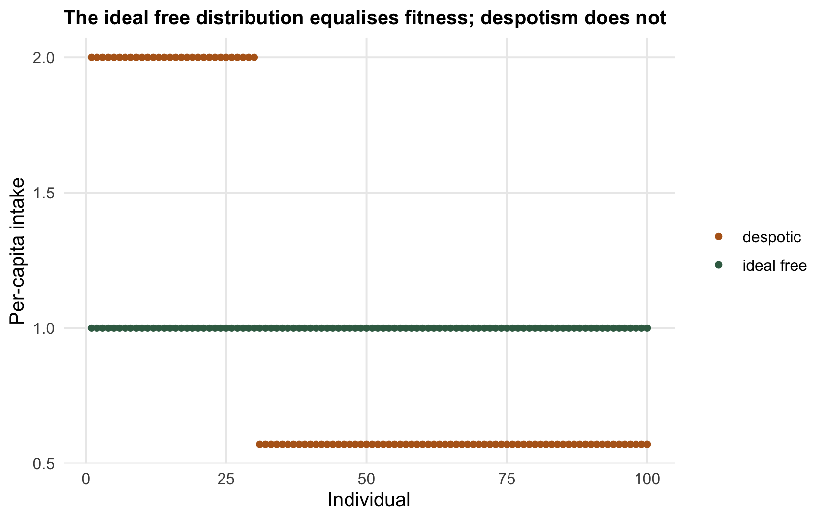
The ideal free model assumes every animal is an interchangeable competitor. Real animals are not: dominants exclude subordinates from the best patches, and the result is a **despotic** distribution (Fretwell and Lucas's own alternative; Fretwell and Lucas 1969 Acta Biotheoretica 19(1):16-36). Its signature is exactly what the ideal free distribution forbids, unequal fitness.
```{r despotic}
Qgood <- 60; Qpoor <- 40; N <- 100; n_dom <- 30
ideal_free  <- (Qgood + Qpoor)/N               # everyone equal
despotic <- c(dominants = Qgood/n_dom, subordinates = Qpoor/(N - n_dom))
c(ideal_free_intake = ideal_free, despotic = despotic)
```
Under the ideal free distribution every one of the `r sprintf("%.0f", N)` animals gets an intake of `r sprintf("%.2f", ifd_intake)`. Under a despotic one, `r sprintf("%.0f", n_dom)` dominants keep the good patch to themselves and take `r sprintf("%.2f", desp_dom)` each, while the excluded majority crowd the poor patch and get `r sprintf("%.2f", desp_sub)`. The mean is identical by construction, `r sprintf("%.2f", ifd_intake)` in both, because the same total is shared among the same animals; the spread is not. If dominants also take a larger share within a patch, a despotic distribution can even reproduce input matching in the counts while producing wildly unequal payoffs, so counts alone will not catch it. The check is to look at the variation in fitness among individuals: the coefficient of variation in intake is `r sprintf("%.2f", cv_ifd)` under the ideal free distribution and `r sprintf("%.2f", cv_desp)` under the despotic one, so near zero is consistent with an ideal free distribution, while a large value shows only that payoffs are unequal. Despotic exclusion produces that, but so do competitors of unequal ability that are free to settle anywhere and exclude no one.
```{r fig-despotic}
#| fig-cap: "Per-capita intake across individuals under two distributions. The ideal free distribution (green) equalises intake; the despotic one (ochre) splits it into a dominant few who do well and an excluded majority who do not."
#| fig-alt: "Intake for each individual under two distributions; the ideal free values form a flat line, the despotic values a high group and a low group."
di <- rbind(data.frame(i = 1:N, intake = ideal_free, dist = "ideal free"),
            data.frame(i = 1:N, intake = c(rep(desp_dom, n_dom), rep(desp_sub, N-n_dom)), dist = "despotic"))
ggplot(di, aes(i, intake, colour = dist)) +
  geom_point(size = 1.4) +
  scale_colour_manual(values = c("ideal free" = col_ifd, "despotic" = col_desp)) +
  labs(x = "Individual", y = "Per-capita intake", colour = NULL,
       title = "The ideal free distribution equalises fitness; despotism does not")
```
## Check 3: the slope is not a mechanism
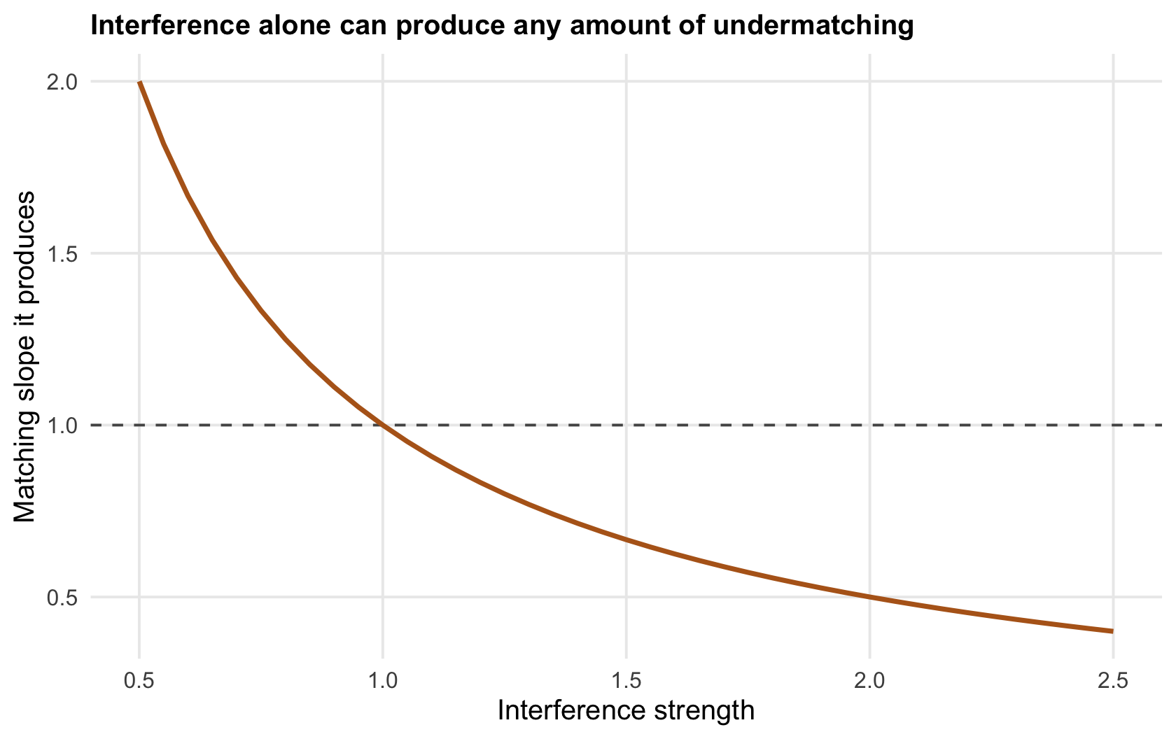
The [matching slope](../input-matching-and-undermatching/) is a summary, and a departure from one is real information, but it cannot be read back into a cause. Interference between foragers, where each one's intake falls as neighbours crowd in, produces a distribution whose matching slope is one over the interference strength (Sutherland 1983 Journal of Animal Ecology 52(3):821-828).
```{r interference}
# with interference of strength m, intake ~ Q * n^(-m); equalising gives n proportional to Q^(1/m)
interference_slope <- function(m) 1/m
sapply(c(0.7, 1.0, 1.5, 2.0), interference_slope)
```
```{r fig-interference}
#| fig-cap: "The matching slope that interference alone produces, against interference strength. Strong interference drives the slope below one, into the same undermatching that weak discrimination and dominance also cause."
#| fig-alt: "A declining curve of matching slope against interference strength, passing through one at an interference exponent of one and falling below it for stronger interference."
dm <- data.frame(m = seq(0.5, 2.5, 0.05)); dm$slope <- 1/dm$m
ggplot(dm, aes(m, slope)) +
  geom_hline(yintercept = 1, colour = col_ref, linetype = "dashed") +
  geom_line(colour = col_desp, linewidth = 1) +
  labs(x = "Interference strength", y = "Matching slope it produces",
       title = "Interference alone can produce any amount of undermatching")
```
Strong interference, an exponent above one, gives a matching slope below one, indistinguishable in the data from the undermatching that weak discrimination or unequal competitors also produce. A slope of one half might mean heavy interference, poor perception, dominance, or an unfinished redistribution, and the number is the same in every case. So the matching slope diagnoses that *something* pulls the distribution off input matching, never *what*; it does not even show that an ideal free assumption has failed, since strong interference alone gives undermatching with the same intake in every patch, a distribution that passes Check 1. Pinning the mechanism down needs an experiment, manipulating patch quality, competitor number, or information, not a better regression.
## What an honest ideal free study looks like
The pattern in these checks is that the ideal free distribution is a null model, not a description. Its job is to say what should happen if animals were ideal, free, and equal, so that the ways real animals depart from it, undermatching, unequal fitness, despotic monopolies, become measurements of the constraints they actually face. Used that way it is one of the most productive ideas in behavioural ecology. Used as a literal account, fitted to counts and never checked against fitness, it is a line that means whatever you want. Measure the fitness it assumes, look at who is competing, and treat the slope as a question rather than an answer.
## References
- Fretwell SD, Lucas HL 1969. Acta Biotheoretica 19(1):16-36 (10.1007/BF01601953).
- Sutherland WJ 1983. Journal of Animal Ecology 52(3):821-828 (10.2307/4456).
## Related tutorials
- [The ideal free distribution](../the-ideal-free-distribution/)
- [Input matching and undermatching](../input-matching-and-undermatching/)
- [Density-dependent habitat selection and isodars](../density-dependent-habitat-selection-isodars/)
- [Resource selection functions](../resource-selection-functions/)