Density-dependent habitat selection

Density-dependent habitat selection and Morris’s isodar in R: how animals spill into poor habitat as density rises, and what the isodar’s slope reveals.

The ideal free distribution equalises intake, moment to moment. But intake is a proxy; what natural selection cares about is fitness, and fitness in a habitat depends on how crowded it is. Turn the ideal free logic on fitness rather than on instantaneous intake and it becomes a tool for reading habitat quality straight off a map of densities, without ever measuring fitness. That tool is the isodar (Morris 1988 Evolutionary Ecology 2(3):253-269).

Spilling from good habitat into poor

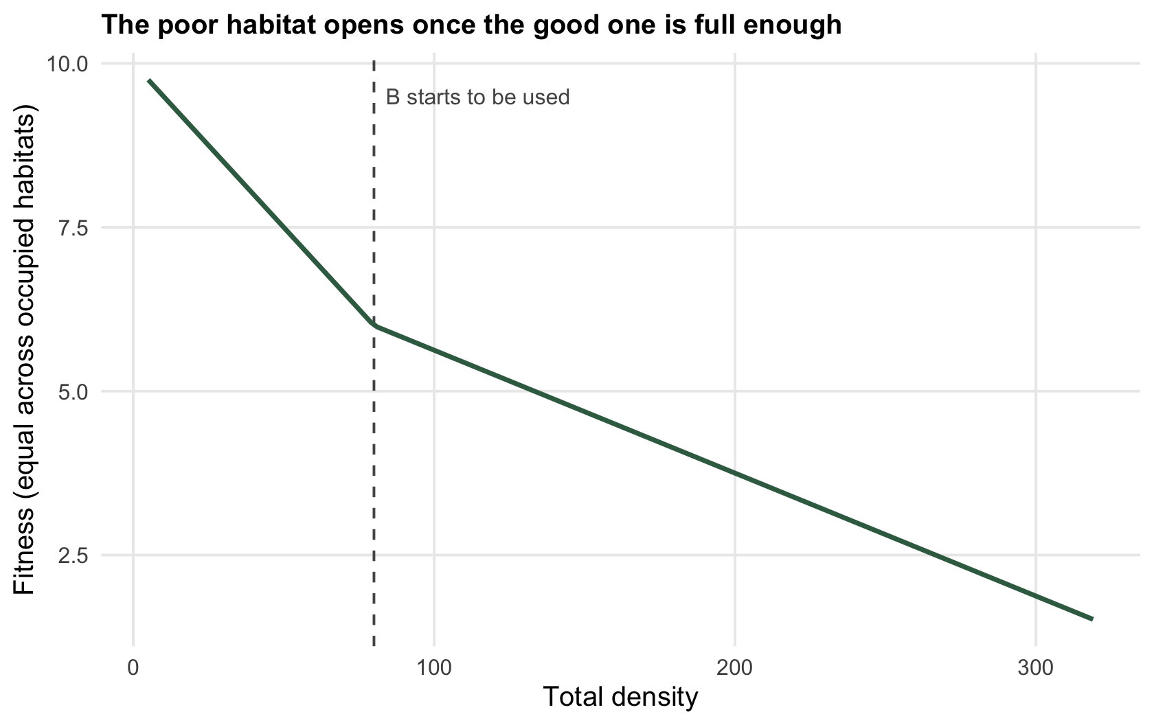
Two habitats, A and B, where fitness falls as density rises. A is better: at the same density it delivers more. An ideal, free animal settles wherever its fitness would be highest, so at low total density everyone crowds into A. As A fills, its fitness drops, and at some point a newcomer would do just as well in empty B as in crowded A. From there on animals split between the two so that fitness stays equal in both.

aA <- 10; bA <- 0.05; aB <- 6; bB <- 0.03     # fitness = a - b * density, habitat A better
WA <- function(n) aA - bA*n; WB <- function(n) aB - bB*n
Nstar <- (aA - aB)/bA                          # total density at which B first gets used
c(spillover_density = Nstar)

spillover_density 
               80 

Below a total density of 80, habitat B stays empty: even packed into A, animals do better there than in an empty B. Above it, they spill into B, and both habitats are occupied at equal fitness thereafter. The spillover threshold is set by how much better A is and how fast it fills.

Wof <- function(N) if (N <= Nstar) WA(N) else WA(ifd_split(N)[1])
dn <- data.frame(N = seq(5, 320, 2)); dn$W <- sapply(dn$N, Wof)
ggplot(dn, aes(N, W)) +
  geom_vline(xintercept = Nstar, colour = col_ref, linetype = "dashed") +
  geom_line(colour = col_A, linewidth = 1) +
  annotate("text", x = Nstar + 4, y = WA(10), label = "B starts to be used", hjust = 0, colour = col_ref, size = 3.4) +
  labs(x = "Total density", y = "Fitness (equal across occupied habitats)",
       title = "The poor habitat opens once the good one is full enough")

Figure 1: Fitness against total density under ideal-free settlement. Below the spillover threshold (dashed) everyone is in A and fitness falls fast; above it, animals split into B and the shared fitness falls more slowly.

The isodar

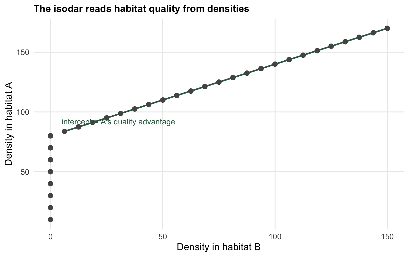
Now the trick. Set the two fitnesses equal, a_A - b_A n_A = a_B - b_B n_B, and solve for the density in A as a function of the density in B. Because the fitness curves are straight lines, the relationship is a straight line too:

\[n_A = \frac{a_A - a_B}{b_A} + \frac{b_B}{b_A}\, n_B .\]

This is the isodar: every combination of densities that leaves an animal indifferent between the habitats. Its two numbers are the whole story. The intercept, 80, is how many animals A holds before B is touched, a measure of how much better A is. The slope, 0.60, is the ratio of the two habitats’ density dependence, how fast B fills relative to A. And the beautiful part is that you can recover both from censuses alone: gather paired densities across sites or years and regress one on the other.

ifd_split <- function(N) if (N <= Nstar) c(N, 0) else {   # ideal-free split of N animals
  nB <- (N - Nstar)/(1 + bB/bA); c(N - nB, nB) }
Ns <- seq(10, 320, 10); sp <- t(sapply(Ns, ifd_split))
occ <- data.frame(nA = sp[,1], nB = sp[,2]); occ <- occ[occ$nB > 0, ]
round(coef(lm(nA ~ nB, data = occ)), 2)

(Intercept)          nB 
       80.0         0.6 

Regressing the density in A on the density in B, over the range where both are occupied, returns an intercept of 80 and a slope of 0.60, exactly the quality gap and the density-dependence ratio built into the fitness curves. Two habitat parameters, read off nothing but head counts, because the animals’ own indifference did the measuring.

allpts <- data.frame(nA = sp[,1], nB = sp[,2])
ggplot(allpts, aes(nB, nA)) +
  geom_smooth(data = occ, method = "lm", se = FALSE, colour = col_A, linewidth = 0.9) +
  geom_point(size = 2.4, colour = col_ref) +
  annotate("text", x = 5, y = iso_int + 12, label = "intercept = A's quality advantage",
           hjust = 0, colour = col_A, size = 3.4) +
  labs(x = "Density in habitat B", y = "Density in habitat A",
       title = "The isodar reads habitat quality from densities")

Figure 2: The isodar. Below the spillover density B is empty (points on the axis); above it, paired densities fall on a straight line whose intercept is A’s quality advantage and whose slope is the density-dependence ratio.

Reading it, and its one big assumption

The isodar is popular in field ecology because it asks so little: no fitness measurements, no marking, just counts in two habitats over a range of total densities. Its slope and intercept classify the habitats, a slope of one means the habitats share the same density dependence and differ only in quality, a steep or shallow slope flags one habitat filling faster than the other, and the intercept ranks them. But all of this rests on one assumption, that the animals are actually distributing themselves by equalising fitness, ideally and freely. If they are not, if movement is constrained, competitors unequal, or the good habitat defended, the line you fit is still a line, but it no longer means what the isodar says it means. Knowing when to trust it is the checking post, and the pattern it produces, density that tracks quantity rather than quality, is the same lesson that runs through source-sink dynamics.

Related tutorials

• The ideal free distribution
• Input matching and undermatching
• Checking an ideal free analysis
• Source-sink population dynamics

References

• Fretwell SD, Lucas HL 1969. Acta Biotheoretica 19(1):16-36 (10.1007/BF01601953).
• Morris DW 1988. Evolutionary Ecology 2(3):253-269 (10.1007/BF02214286).