---
title: "Source-sink population dynamics"
description: "Source-sink dynamics in R: the BIDE budget, why a sink population persists only on immigration from a source, and what the local growth rate really measures."
date: "2026-07-02 10:00"
date-modified: "2026-10-07"
categories: [ecology tutorial, R, population ecology, conservation, metapopulations]
image: thumbnail.png
image-alt: "A sink population collapsing to zero when isolated but rising to a stable level when subsidised by immigration from a source."
---
*Corrected 7 October 2026: the post said that counting animals tells you almost nothing about habitat quality; it now says that a count on its own can mislead about habitat quality.*
```{r setup}
#| code-fold: true
#| code-summary: "Setup: packages, colours and plot theme"
#| results: hide
#| message: false
#| warning: false
knitr::opts_chunk$set(echo = TRUE, message = FALSE, warning = FALSE,
                      dev = "png", dpi = 120, fig.path = "figures/",
                      fig.width = 7, fig.height = 4.4)
library(ggplot2)
theme_te <- theme_minimal(base_size = 12) +
  theme(panel.background = element_rect(fill = "#f5f4ee", colour = NA),
        plot.background  = element_rect(fill = "#f5f4ee", colour = NA),
        panel.grid.minor = element_blank(),
        plot.title = element_text(face = "bold", size = 12))
theme_set(theme_te)
col_alone <- "#b5651d"; col_sub <- "#3a6b52"; col_ref <- "#555555"

lam <- function(PA, PJ, b) PA + PJ * b
l1 <- lam(0.6, 0.3, 3.0)   # source
l2 <- lam(0.6, 0.3, 0.8)   # sink
n1 <- 100
n2_eq <- n1 * (l1 - 1) / (1 - l2)
years <- 40; surplus <- n1 * (l1 - 1)
Na <- numeric(years+1); Ns <- numeric(years+1); Na[1] <- Ns[1] <- 80
for (t in 2:(years+1)) { Na[t] <- Na[t-1]*l2; Ns[t] <- Ns[t-1]*l2 + surplus }
```
A basic idea in population ecology is that habitat quality varies, but the consequences of that idea are strange enough that they still catch people out. In a good patch, births outnumber deaths and the population would grow on its own. In a poor patch, deaths outnumber births and the population would dwindle to nothing if left alone. The good patch, a source, exports its surplus; the poor patch, a sink, survives only on those exports. Pulliam 1988 The American Naturalist 132(5):652-661 laid this out, and it changes what a population count is worth.
## The BIDE budget
A local population changes through four flows: Births, Immigration, Deaths, Emigration. Collapse births and deaths into a local finite growth rate, the factor a population multiplies by each year without any movement. For a simple annual life it is adult survival plus juvenile survival times fecundity.
```{r lambda}
lam <- function(PA, PJ, b) PA + PJ * b   # adult survival + juvenile survival * fecundity
c(source = lam(0.6, 0.3, 3.0), sink = lam(0.6, 0.3, 0.8))
```
The source has a local growth rate above one, `r sprintf("%.2f", l1)`: without any immigration it would grow, so its births more than replace its deaths and the extra individuals must go somewhere. The sink has a local growth rate below one, `r sprintf("%.2f", l2)`: without immigration it shrinks every year. A sink is not a small population or a rare one; it is a population that cannot replace itself.
## A sink lives on subsidy
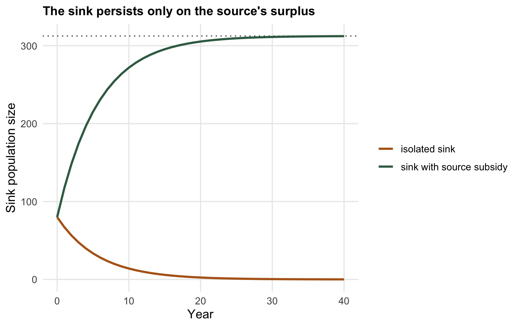
Take a sink and follow it two ways: isolated, and receiving the surplus that a source of `r sprintf("%.0f", n1)` breeding adults sends out each year.
```{r dynamics}
l2 <- lam(0.6, 0.3, 0.8); surplus <- 100 * (lam(0.6, 0.3, 3.0) - 1)
sink_alone <- Reduce(function(N, .) N * l2,             1:40, accumulate = TRUE, 80)
sink_subs  <- Reduce(function(N, .) N * l2 + surplus,   1:40, accumulate = TRUE, 80)
c(alone_final = tail(sink_alone, 1), subsidised_final = tail(sink_subs, 1))
```
Isolated, the sink falls from `r sprintf("%.0f", 80)` toward zero, reaching `r sprintf("%.1f", Na[years+1])` after forty years: local extinction, exactly as a growth rate below one demands. Fed the source's surplus, the same sink climbs and settles at `r sprintf("%.0f", n2_eq)`. The inflow of `r sprintf("%.0f", surplus)` immigrants a year exactly balances the annual shortfall between births and deaths. Cut the source and the sink is gone; the persistence you see is borrowed.
```{r fig-dynamics}
#| fig-cap: "A sink population over forty years. Isolated (ochre) it collapses to local extinction; subsidised by a source's surplus (green) it rises to a stable level held up entirely by immigration."
#| fig-alt: "Two trajectories of a sink population; the isolated one declines toward zero, the subsidised one rises and levels off at a stable positive size."
d <- rbind(data.frame(t = 0:years, N = Na, kind = "isolated sink"),
           data.frame(t = 0:years, N = Ns, kind = "sink with source subsidy"))
ggplot(d, aes(t, N, colour = kind)) +
  geom_hline(yintercept = n2_eq, colour = col_ref, linetype = "dotted") +
  geom_line(linewidth = 1) +
  scale_colour_manual(values = c("isolated sink" = col_alone, "sink with source subsidy" = col_sub)) +
  labs(x = "Year", y = "Sink population size", colour = NULL,
       title = "The sink persists only on the source's surplus")
```
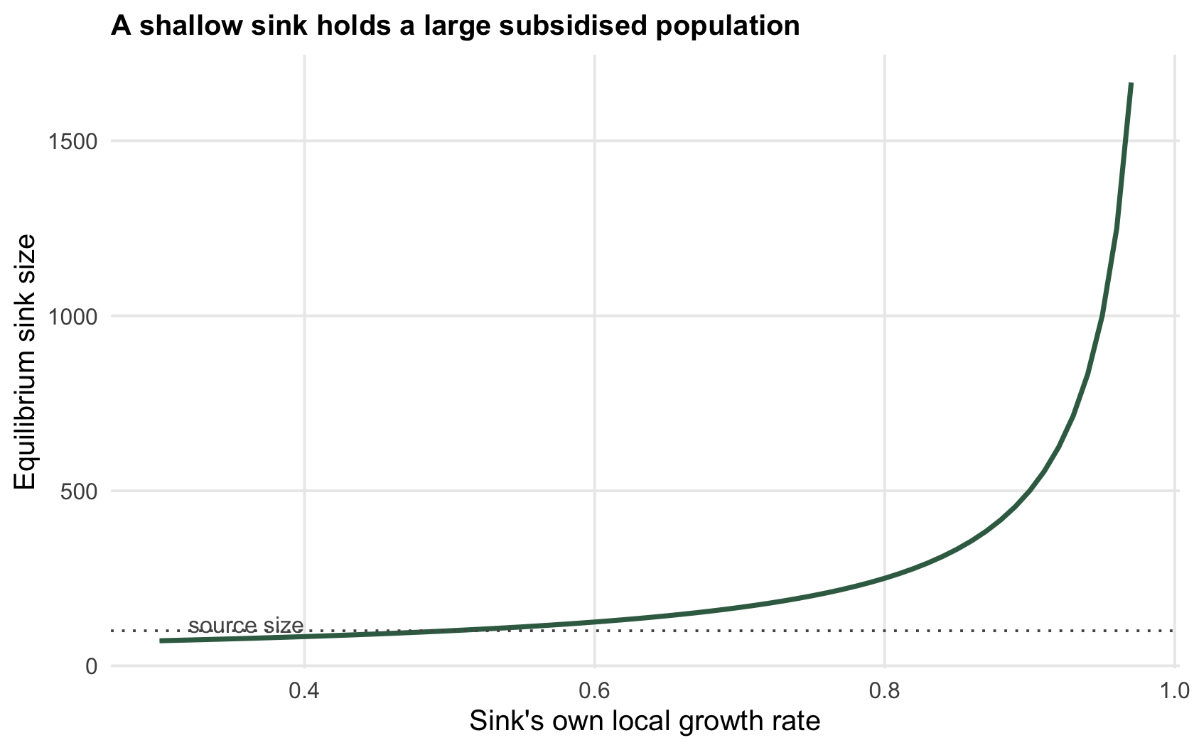
How large that subsidised population settles depends on how deep a sink it is. A shallow sink, one whose local growth rate is only just below one, loses very little each year, so the same immigration piles up into a large standing population; a severe sink burns through immigrants fast and stays small.
```{r fig-equilibrium}
#| fig-cap: "Equilibrium sink size against the sink's own local growth rate, for a fixed source surplus. As the sink's growth rate approaches one, the same immigration supports an ever larger population."
#| fig-alt: "A rising curve of equilibrium sink size against the sink's local growth rate, climbing steeply as the growth rate approaches one."
l2g <- seq(0.3, 0.97, 0.01)
de <- data.frame(l2 = l2g, n2 = surplus / (1 - l2g))
ggplot(de, aes(l2, n2)) +
  geom_line(colour = col_sub, linewidth = 1) +
  geom_hline(yintercept = n1, colour = col_ref, linetype = "dotted") +
  annotate("text", x = 0.32, y = n1, label = "source size", hjust = 0, vjust = -0.6, colour = col_ref, size = 3.4) +
  labs(x = "Sink's own local growth rate", y = "Equilibrium sink size",
       title = "A shallow sink holds a large subsidised population")
```
## What the local growth rate does and does not tell you
The local growth rate is a statement about self-sufficiency: above one, the habitat can stand alone; below one, it cannot. It is not a statement about size, and this is where intuition fails. A sink can be crowded, holding far more animals than the source that feeds it, because the source keeps pushing its surplus downhill into the sink. It is not a statement about importance either: a sink can be a population trap that drains the source, or a valuable stepping stone, depending on the flows. A [companion post](../sinks-can-hold-high-density/) shows how a sink comes to hold more individuals than its source, which is why a count on its own can mislead about habitat quality, and the [checking post](../checking-a-source-sink-analysis/) shows what you have to measure instead.
## References
- Pulliam HR 1988. The American Naturalist 132(5):652-661 (10.1086/284880).
## Related tutorials
- [Sinks can hold high density](../sinks-can-hold-high-density/)
- [Ecological traps and pseudo-sinks](../ecological-traps-and-pseudo-sinks/)
- [Checking a source-sink analysis](../checking-a-source-sink-analysis/)
- [The Levins metapopulation model](../the-levins-metapopulation-model/)