---
title: "Ecological traps and pseudo-sinks"
description: "Two ways a sink deceives, in R: an ecological trap that lures settlers into poor habitat, and a pseudo-sink that looks doomed but persists when isolated."
date: "2026-07-02 11:00"
date-modified: "2026-10-15"
categories: [ecology tutorial, R, population ecology, conservation, habitat selection]
image: thumbnail.png
image-alt: "Local growth rate against density for a true sink below one everywhere and a pseudo-sink above one at low density, crossing one at its own carrying capacity."
---
*Corrected 15 October 2026: the post said the three cases can be told apart only from the local demography and the settlement behaviour, not from counts; local births and deaths at the crowded density make a pseudo-sink look like a sink too, so the sentence now says it takes how the local demography responds when the density falls, as in the isolation test, together with the settlement behaviour, and rules out a single headcount.*
*Corrected 7 October 2026: the post defined an ecological trap as a genuine sink that animals prefer; the cited definition is a poor habitat that animals prefer over better habitat available to them, with no requirement that it be a sink, and the sentence now gives that definition, while the trap in this post is still a sink.*
```{r setup}
#| code-fold: true
#| code-summary: "Setup: packages, colours and plot theme"
#| results: hide
#| message: false
#| warning: false
knitr::opts_chunk$set(echo = TRUE, message = FALSE, warning = FALSE,
                      dev = "png", dpi = 120, fig.path = "figures/",
                      fig.width = 7, fig.height = 4.4)
library(ggplot2)
theme_te <- theme_minimal(base_size = 12) +
  theme(panel.background = element_rect(fill = "#f5f4ee", colour = NA),
        plot.background  = element_rect(fill = "#f5f4ee", colour = NA),
        panel.grid.minor = element_blank(),
        plot.title = element_text(face = "bold", size = 12))
theme_set(theme_te)
col_true <- "#b5651d"; col_pseudo <- "#3a6b52"; col_ref <- "#555555"

lam_true   <- function(N) rep(0.85, length(N))
lam_pseudo <- function(N) pmax(1.6 - 0.006*N, 0.01)
iso <- function(lam, N0, yr = 40) { N <- N0; for (t in 1:yr) N <- N * lam(N); N }
true_iso <- iso(lam_true, 180); pseudo_iso <- iso(lam_pseudo, 180)
```
A habitat that receives more immigrants than it exports, and whose population would fall without them, is the textbook signature of a sink. But two very different situations produce that same signature, and confusing them leads to opposite conservation mistakes. One is a habitat so attractive that animals pour into it even though it is killing them. The other is a perfectly good habitat that only looks like a sink because it is overcrowded. This post separates the ecological trap from the pseudo-sink.
## The pseudo-sink: good habitat wearing a sink's disguise
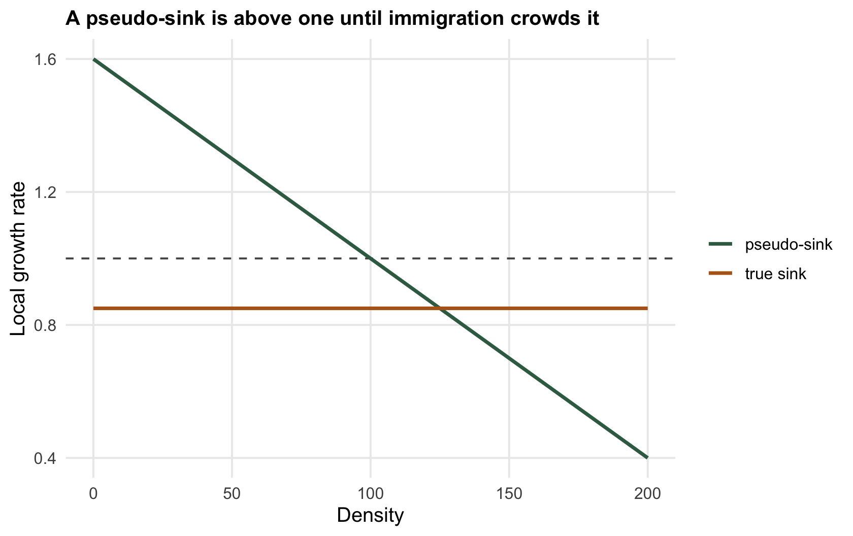
Start with the reassuring case. A **pseudo-sink** (Watkinson and Sutherland 1995 Journal of Animal Ecology 64(1):126-130) is a habitat whose local growth is density-dependent and genuinely good, but which receives so much immigration that it is pushed above its own carrying capacity. Crowded past capacity, its local growth rate drops below one, and a snapshot calls it a sink. Contrast it with a **true sink**, where the growth rate is below one at every density, immigration or no.
```{r sinks}
lam_true   <- function(N) rep(0.85, length(N))          # below one at every density
lam_pseudo <- function(N) pmax(1.6 - 0.006*N, 0.01)     # good, but density-dependent
rbind(at_crowded_180 = c(true = lam_true(180), pseudo = lam_pseudo(180)),
      at_sparse_10   = c(true = lam_true(10),  pseudo = lam_pseudo(10)))
```
At an immigration-inflated density of `r sprintf("%.0f", 180)`, both look like sinks: the true sink at `r sprintf("%.2f", lam_true(180))` and the pseudo-sink even lower at `r sprintf("%.2f", lam_pseudo(180))`. Drop the density to `r sprintf("%.0f", 10)` and they part company: the true sink is still `r sprintf("%.2f", lam_true(10))`, below one, while the pseudo-sink is `r sprintf("%.2f", lam_pseudo(10))`, comfortably above. The test that settles it is to cut the immigration and watch.
```{r isolate}
iso <- function(lam, N0, yr = 40) { N <- N0; for (t in 1:yr) N <- N * lam(N); N }
c(true_sink_isolated = iso(lam_true, 180), pseudo_sink_isolated = iso(lam_pseudo, 180))
```
Isolated from a starting `r sprintf("%.0f", 180)`, the true sink collapses to `r sprintf("%.1f", true_iso)`, extinct, while the pseudo-sink relaxes down to its own carrying capacity of `r sprintf("%.0f", pseudo_iso)` and persists indefinitely. Write off a true sink and you lose little; write off a pseudo-sink and you have abandoned good habitat because a headcount was crowded.
```{r fig-pseudo}
#| fig-cap: "Local growth rate against density. The true sink (ochre) is below one everywhere. The pseudo-sink (green) is above one until immigration crowds it past its own carrying capacity, where it crosses one; isolated it settles there and persists."
#| fig-alt: "Two curves of local growth rate against density; the ochre true-sink line is flat below one, the green pseudo-sink line slopes down and crosses one at its carrying capacity."
Ng <- seq(0, 200, 1)
d <- rbind(data.frame(N = Ng, lam = lam_true(Ng),   kind = "true sink"),
           data.frame(N = Ng, lam = lam_pseudo(Ng), kind = "pseudo-sink"))
ggplot(d, aes(N, lam, colour = kind)) +
  geom_hline(yintercept = 1, colour = col_ref, linetype = "dashed") +
  geom_line(linewidth = 1) +
  scale_colour_manual(values = c("true sink" = col_true, "pseudo-sink" = col_pseudo)) +
  labs(x = "Density", y = "Local growth rate", colour = NULL,
       title = "A pseudo-sink is above one until immigration crowds it")
```
## The ecological trap: attractive and lethal
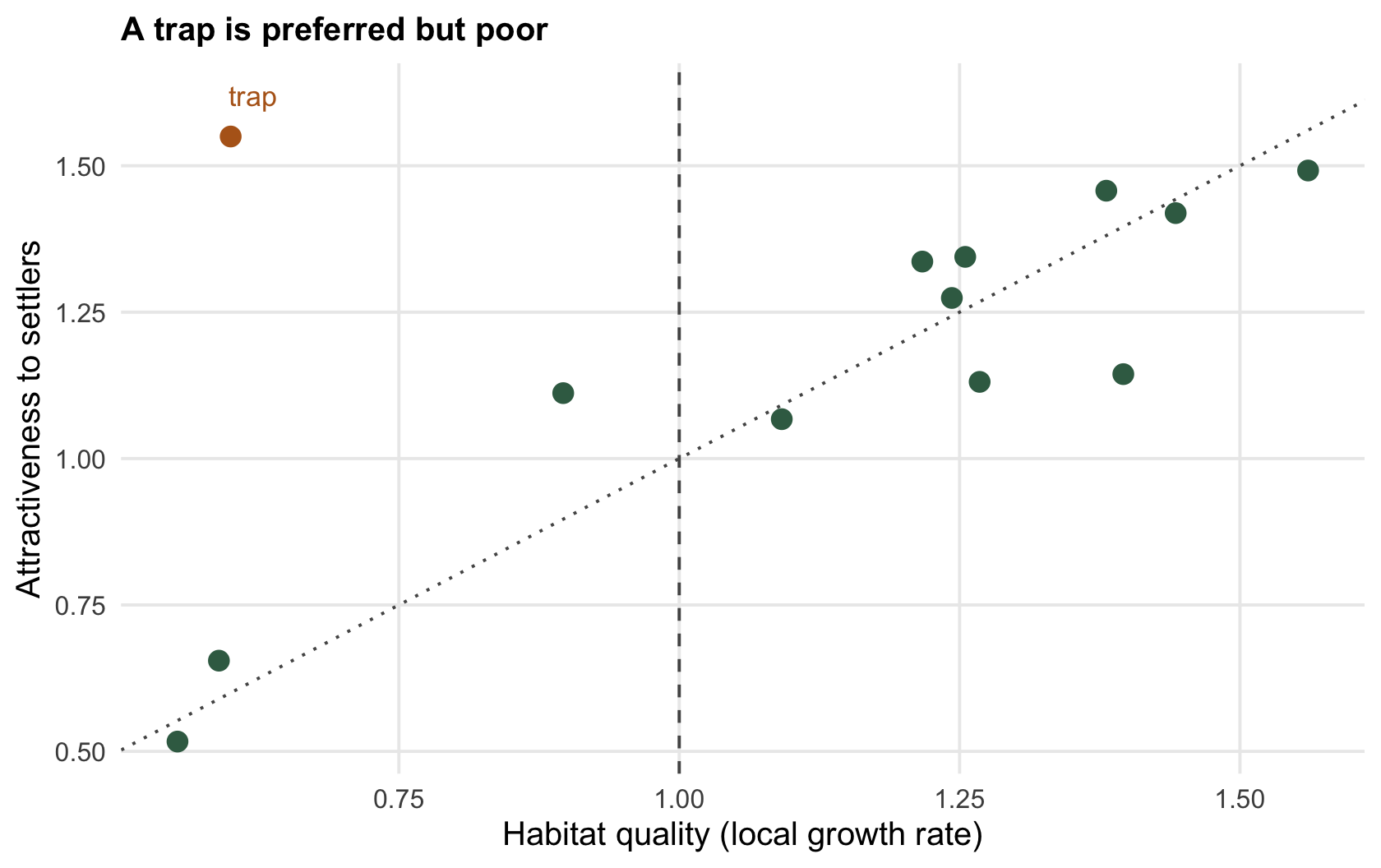
The other deception runs the opposite way. An **ecological trap** is a poor habitat, in this post a sink, that animals actively *prefer* over better habitat available to them (Schlaepfer et al. 2002 Trends in Ecology and Evolution 17(10):474-480; Battin 2004 Conservation Biology 18(6):1482-1491). Habitat choice evolved to track cues that once predicted quality, and when human change breaks the link between cue and quality, the cue can point the wrong way: a freshly mown field that signals lush grassland, asphalt that polarises light like water, a forest edge that looks safe but concentrates predators. Settlers choose the trap over better habitat and pay for it.
A trap is worse than an ordinary sink, because an ordinary sink is at least avoided when better options exist, whereas a trap pulls animals *out* of sources. Plotting habitats by their quality and their attractiveness makes the danger zone explicit: quality and preference should rise together, and a trap is the habitat that sits where they come apart, high preference, low quality.
```{r fig-trap}
#| fig-cap: "Habitats in quality-preference space. Along the diagonal, preference tracks quality. A trap (ochre) sits off it: highly preferred but poor quality, drawing settlers away from the genuine sources."
#| fig-alt: "A scatter of habitats plotted by quality and preference; most lie near a rising diagonal, but one labelled trap sits at high preference and low quality."
set.seed(409)
q <- runif(12, 0.4, 1.6); pref <- pmin(pmax(q + rnorm(12, 0, 0.12), 0.2), 1.7)
hab <- data.frame(quality = q, preference = pref, type = "matched")
hab <- rbind(hab, data.frame(quality = 0.6, preference = 1.55, type = "trap"))
ggplot(hab, aes(quality, preference, colour = type)) +
  geom_abline(slope = 1, intercept = 0, colour = col_ref, linetype = "dotted") +
  geom_vline(xintercept = 1, colour = col_ref, linetype = "dashed") +
  geom_point(size = 3) +
  annotate("text", x = 0.62, y = 1.62, label = "trap", colour = col_true, size = 3.6) +
  scale_colour_manual(values = c("matched" = col_pseudo, "trap" = col_true), guide = "none") +
  labs(x = "Habitat quality (local growth rate)", y = "Attractiveness to settlers",
       title = "A trap is preferred but poor")
```
## Three diagnoses, three responses
The management response depends entirely on which of the three you have. A true sink is low-quality habitat that animals rightly avoid when they can; often it can be left alone. A pseudo-sink is good habitat that a headcount slandered; protect it. A trap is low-quality habitat that animals wrongly love, and it is the dangerous one, because it drains the sources and can pull the whole population down; the response is to fix the cue, remove the attractive lure or restore the quality behind it. Telling them apart cannot be done from a headcount or from occupancy, nor from local births and deaths at the crowded density, which make a pseudo-sink look like a sink too; it takes how the local demography responds when the density falls, as in the isolation test above, together with the settlement behaviour, which is where the [checking post](../checking-a-source-sink-analysis/) goes next.
## References
- Battin J 2004. Conservation Biology 18(6):1482-1491 (10.1111/j.1523-1739.2004.00417.x).
- Schlaepfer MA et al. 2002. Trends in Ecology and Evolution 17(10):474-480 (10.1016/S0169-5347(02)02580-6).
- Watkinson AR, Sutherland WJ 1995. Journal of Animal Ecology 64(1):126-130 (10.2307/5833).
## Related tutorials
- [Source-sink population dynamics](../source-sink-dynamics/)
- [Why sinks hold high density](../sinks-can-hold-high-density/)
- [Checking a source-sink analysis](../checking-a-source-sink-analysis/)
- [Extinction risk and population viability analysis](../extinction-risk-pva/)