Checking a source-sink analysis

Three checks for a source-sink study in R: why counts mislead, separating local recruits from immigrants, and defining a source by contribution not just growth.

Everything in this series has been a warning that a sink does not look like a sink. It can be crowded, it can be preferred, it can be excellent habitat having a bad year. So how do you actually tell a source from a sink? Not from the things easiest to measure. These three checks are about what to measure instead, and each rules out a tempting shortcut.

Check 1: counts and occupancy cannot classify a habitat

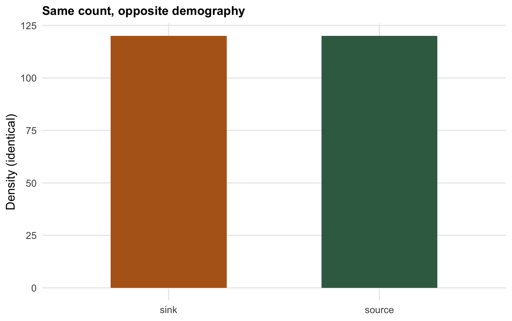
The first check is really a prohibition. Source and sink are defined by the local balance of births and deaths, and that balance is invisible in a headcount. Two habitats can hold identical numbers, be equally occupied year after year, and be demographic opposites.

source_hab <- c(density = 120, births = 0.9, deaths = 0.5)   # births > deaths: a source
sink_hab   <- c(density = 120, births = 0.4, deaths = 0.8)   # deaths > births: a sink
rbind(source = source_hab, sink = sink_hab)

       density births deaths
source     120    0.9    0.5
sink       120    0.4    0.8

Both habitats hold 120 animals. The first has births outrunning deaths and is a source; the second has deaths outrunning births and is a sink held up by immigration. A survey that records density, or presence and absence, sees two identical habitats. Occupancy models, distribution maps, and abundance counts, the workhorses of monitoring, are all blind to the distinction, because the distinction lives in the vital rates, not the numbers.

d <- data.frame(habitat = c("source", "sink"), density = c(120, 120), kind = c("source", "sink"))
ggplot(d, aes(habitat, density, fill = kind)) +
  geom_col(width = 0.55) +
  scale_fill_manual(values = c("source" = col_source, "sink" = col_sink), guide = "none") +
  labs(x = NULL, y = "Density (identical)", title = "Same count, opposite demography")

Figure 1: Two habitats with the same density and occupancy, one a source and one a sink. A count cannot separate them; only the birth and death rates can.

Check 2: are the recruits local, or immigrants?

Suppose you do measure vital rates by counting young. A subtler trap waits: the young and the newcomers in a habitat are a mix of locally-produced individuals and immigrants, and if you credit them all to local reproduction you inflate the local growth rate and can promote a sink to a source. The cleanest way to see it is to compute growth the way a monitoring programme would, from year-to-year counts, at a sink sitting at its stable equilibrium.

l_local <- 0.84; imm <- 48                 # true local growth rate, and annual immigrants
n_sink  <- imm/(1 - l_local)               # equilibrium sink size
apparent <- (n_sink*l_local + imm)/n_sink  # growth inferred from total counts
c(true_local_lambda = l_local, apparent_lambda_from_counts = apparent, sink_size = n_sink)

          true_local_lambda apparent_lambda_from_counts 
                       0.84                        1.00 
                  sink_size 
                     300.00 

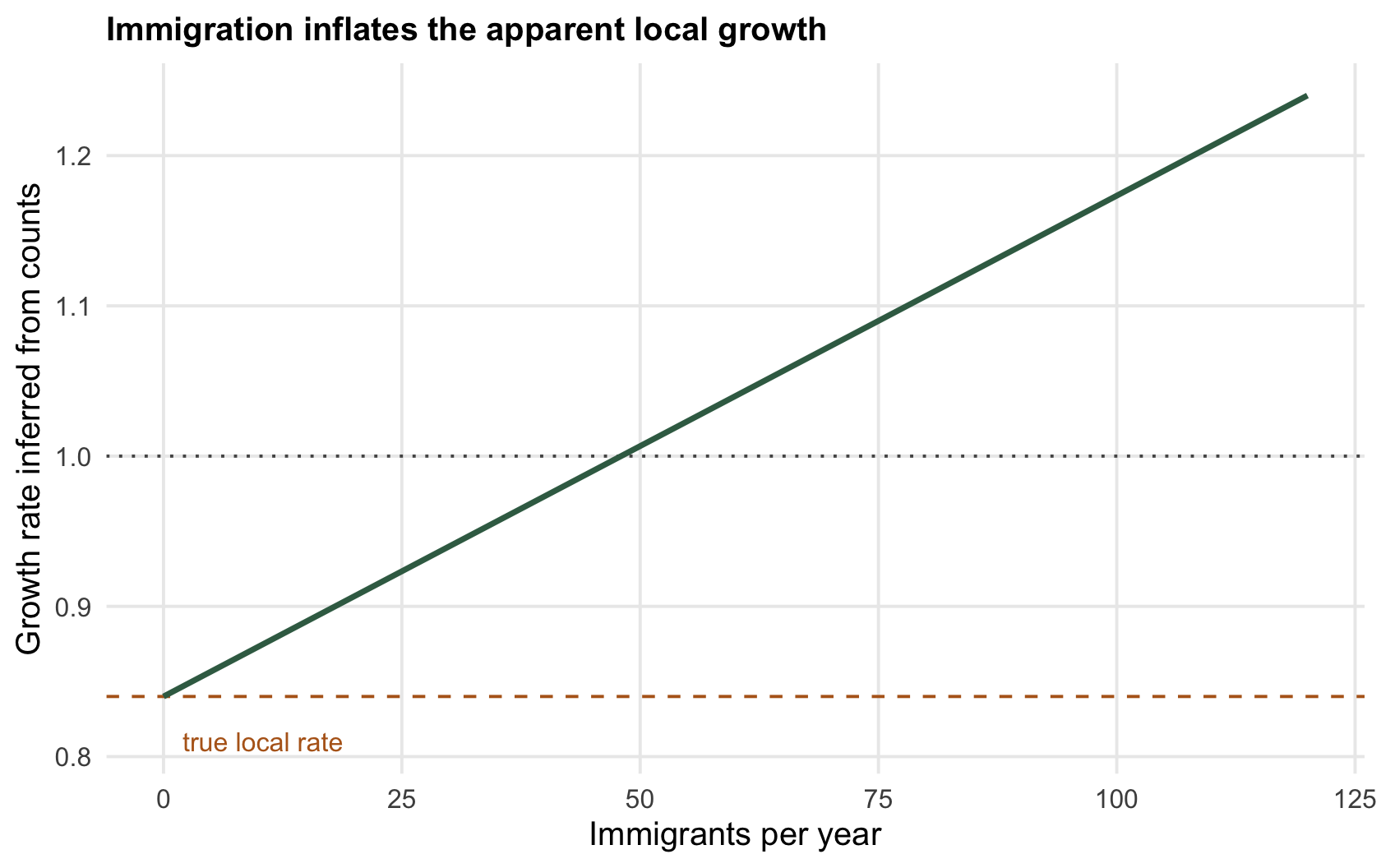
The true local growth rate is 0.84: a sink. But at equilibrium the counts are steady, so growth inferred from the total, next year’s count over this year’s, is 1.00, exactly one. A monitoring programme watching the numbers would conclude the population is stable and self-sustaining, when in fact it is a sink kept level by 48 immigrants a year. Only by marking individuals, or using natal-origin markers like genetics or isotopes, can you separate the animals this habitat produced from the ones it merely received, and only that separation gives the local growth rate.

The size of the illusion grows with the subsidy. For a sink held at a fixed size, the more immigrants arrive, the higher the growth rate a count-based analysis reports, until it climbs past one and the sink is misread as a thriving source.

N0 <- 300
di <- data.frame(imm = seq(0, 120, 2))
di$apparent <- (N0*l_local + di$imm)/N0
ggplot(di, aes(imm, apparent)) +
  geom_hline(yintercept = 1, colour = col_ref, linetype = "dotted") +
  geom_hline(yintercept = l_local, colour = col_sink, linetype = "dashed") +
  geom_line(colour = col_source, linewidth = 1) +
  annotate("text", x = 2, y = l_local - 0.03, label = "true local rate", hjust = 0, colour = col_sink, size = 3.4) +
  labs(x = "Immigrants per year", y = "Growth rate inferred from counts",
       title = "Immigration inflates the apparent local growth")

Figure 2: Growth rate inferred from counts, against the number of immigrants arriving at a sink of fixed size. The true local rate (dashed) stays below one; the count-based rate climbs through one as immigration rises.

Check 3: is “source” the same as “important”?

The last check is conceptual. It is tempting to define a source as any habitat with a local growth rate above one and stop there, but that conflates self-sufficiency with contribution. What a habitat is worth to the wider landscape is the surplus it actually sends out that recruits elsewhere, and two self-sufficient habitats can differ enormously in that.

# two sources, both self-sufficient (lambda > 1), very different net contributions
sA <- c(lambda = 1.20, size = 40);  sB <- c(lambda = 1.04, size = 400)
c(A_emigrants = sA["size"]*(sA["lambda"]-1), B_emigrants = sB["size"]*(sB["lambda"]-1))

A_emigrants.size B_emigrants.size 
               8               16 

Source A has the higher local growth rate, 1.20, and by the simple definition is the “better” source. But it is small, so it exports 8 surplus animals a year. Source B grows only just above replacement yet is large, and exports 16, four times as many. Ranked by per-capita growth, A wins; ranked by contribution to the landscape, B wins. Runge et al. 2006 The American Naturalist 167(6):925-938 formalised this, defining a habitat’s role by its net contribution through reproductive value rather than by its local growth rate alone. For deciding where conservation effort goes, contribution is the currency, not the local rate.

What a real classification needs

The through-line of all three checks is that source-sink status is a demographic claim, and demographic claims need demographic data: local survival and fecundity, partitioned from immigration by marked individuals, and read as contribution to the landscape rather than as a local rate in isolation. That is why the question is usually answered with capture-recapture and integrated population models, not with the abundance surveys that first raised it. When a study labels a habitat a source or a sink from counts, occupancy, or density alone, it has not measured the thing the label names.

Related tutorials

• Source-sink population dynamics
• Why sinks hold high density
• Ecological traps and pseudo-sinks
• Integrated population model basics

References

• Pulliam HR 1988. The American Naturalist 132(5):652-661 (10.1086/284880).
• Runge JP, Runge MC, Nichols JD 2006. The American Naturalist 167(6):925-938 (10.1086/503531).