---
title: "Input matching and undermatching"
description: "Testing the ideal free distribution in R: the matching slope, why real animals undermatch and under-use the best patches, and what that slope really reveals."
date: "2026-07-03 10:00"
date-modified: "2026-10-15"
categories: [ecology tutorial, R, foraging, behaviour, habitat selection]
image: thumbnail.png
image-alt: "A log-log plot of foragers against resources with a matching line of slope one and a shallower undermatching line that sits above it in the poor patches and crosses to below it in the richest ones."
---
*Corrected 15 October 2026: the post said that the matching slope reports how sharply animals distinguish good patches from bad, and that a slope of one half fits foragers that cannot see the difference between patches; it now says that the first holds in this model, where discrimination is the only departure from matching, and that the second fits foragers that only partly see the difference. It also said that a departure from matching shows an ideal free assumption relaxed somewhere; it now says that interference alone can produce one among ideal, free foragers.*
*Corrected 7 October 2026: the post cited Sutherland's paper for dominant competitors monopolising the best patch; that paper models interference between foragers, so the citation now sits with heavy interference in the list of mechanisms.*
```{r setup}
#| code-fold: true
#| code-summary: "Setup: packages, colours and plot theme"
#| results: hide
#| message: false
#| warning: false
knitr::opts_chunk$set(echo = TRUE, message = FALSE, warning = FALSE,
                      dev = "png", dpi = 120, fig.path = "figures/",
                      fig.width = 7, fig.height = 4.4)
library(ggplot2)
theme_te <- theme_minimal(base_size = 12) +
  theme(panel.background = element_rect(fill = "#f5f4ee", colour = NA),
        plot.background  = element_rect(fill = "#f5f4ee", colour = NA),
        panel.grid.minor = element_blank(),
        plot.title = element_text(face = "bold", size = 12))
theme_set(theme_te)
col_match <- "#3a6b52"; col_under <- "#b5651d"; col_ref <- "#555555"

set.seed(412)
Q <- c(40, 30, 20, 10); N <- 200
settle <- function(s) as.numeric(rmultinom(1, N, Q^s / sum(Q^s)))
slope_of <- function(n) unname(coef(lm(log(n) ~ log(Q)))[2])
avg_slope <- function(s) mean(replicate(300, slope_of(settle(s))))
sl_perfect <- avg_slope(1.0); sl_under <- avg_slope(0.5)
```
The ideal free distribution predicts [input matching](../the-ideal-free-distribution/): the number of foragers in a patch should be proportional to its resource supply. That is a testable line, and testing it turns the whole theory into a single number, the matching slope. What that number keeps coming out to is one of the most consistent results in behavioural ecology, and it is not one.
## The matching slope
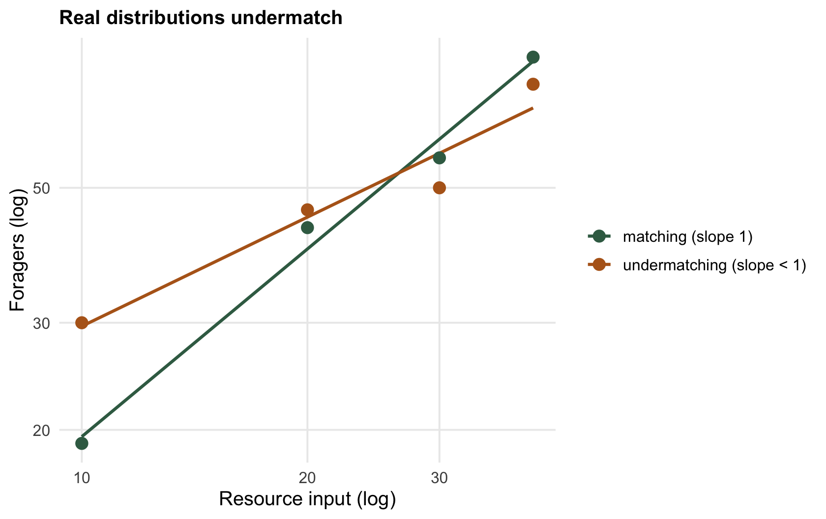
Proportionality is a straight line through the origin, which on logarithmic axes becomes a line of slope one. So plot the log of the number of foragers in each patch against the log of its resource input, fit a line, and read the slope. A slope of one is perfect matching. A slope below one is **undermatching**: the rich patches hold fewer foragers than proportionality demands, and the poor patches hold more. A slope above one is overmatching, and is rare.
```{r slope}
Q <- c(40, 30, 20, 10); N <- 200
settle   <- function(s) as.numeric(rmultinom(1, N, Q^s / sum(Q^s)))  # s is discrimination
slope_of <- function(n) unname(coef(lm(log(n) ~ log(Q)))[2])
set.seed(412)
c(perfect_discrimination = slope_of(settle(1.0)), imperfect = slope_of(settle(0.5)))
```
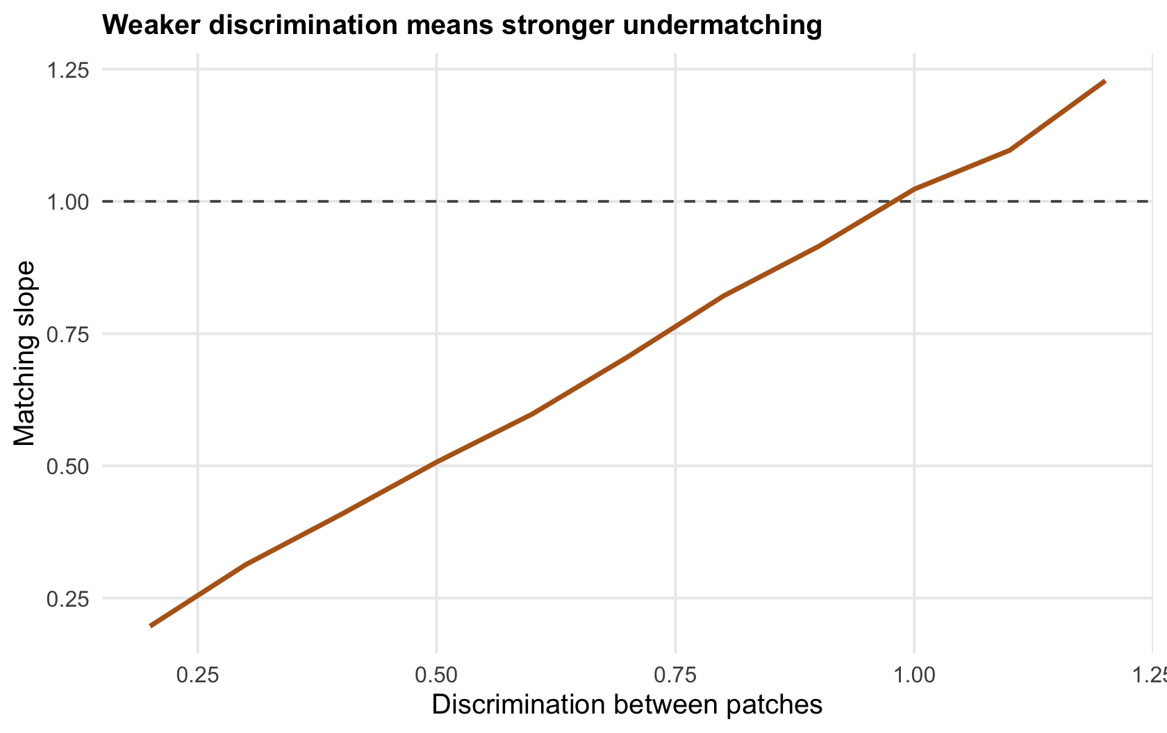
Here foragers settle in each patch with a probability that depends on the patch's richness raised to a power `s`, a discrimination parameter: at `s` of one they weight patches exactly by richness, below one they blur the differences. Averaged over many realisations the matching slope comes out at `r sprintf("%.2f", sl_perfect)` when discrimination is perfect and `r sprintf("%.2f", sl_under)` when it is halved. Four patches make a very noisy regression, which is why the single draw printed above sits well away from both averages. In this model, where discrimination is the only thing pulling the animals off matching, the slope essentially reports how sharply they distinguish good patches from bad.
```{r fig-slope}
#| fig-cap: "Foragers against resources on log axes. Perfect matching lies on the slope-one line (green); real distributions are shallower (ochre), with the poorest patches over-used and the best under-used."
#| fig-alt: "Log-log scatter of foragers against resources with a green matching line of slope one and a shallower ochre undermatching line, points below the matching line at high resource values."
set.seed(7)
nm <- settle(1.0); nu <- settle(0.5)
dd <- rbind(data.frame(Q = Q, n = nm, kind = "matching (slope 1)"),
            data.frame(Q = Q, n = nu, kind = "undermatching (slope < 1)"))
ggplot(dd, aes(Q, n, colour = kind)) +
  geom_smooth(method = "lm", se = FALSE, linewidth = 0.9) +
  geom_point(size = 3) +
  scale_x_log10() + scale_y_log10() +
  scale_colour_manual(values = c("matching (slope 1)" = col_match, "undermatching (slope < 1)" = col_under)) +
  labs(x = "Resource input (log)", y = "Foragers (log)", colour = NULL,
       title = "Real distributions undermatch")
```
## Why animals undermatch
Across dozens of experiments, from sticklebacks to ducks to people, the matching slope lands below one far more often than on it (Kennedy and Gray 1993 Oikos 68(1):158-166). The consistency is the clue: something systematic pulls animals off perfect matching, and several mechanisms all pull the same way. Perceptual limits blur the difference between a good and a slightly better patch. Incomplete information means animals sample and lag rather than settling instantly. Travel and switching costs make it not worth chasing a small advantage. And competitors are rarely equal, so a few dominant individuals monopolise the best patch and the rest give up on it sooner than matching would predict. Every one of these leaves the best patch under-used.
```{r fig-discrimination}
#| fig-cap: "The matching slope against how sharply foragers discriminate between patches. Perfect discrimination gives a slope of one; blurring the differences drives the slope down into undermatching."
#| fig-alt: "A rising line of matching slope against a discrimination parameter, passing through slope one at perfect discrimination and falling below one as discrimination weakens."
ss <- seq(0.2, 1.2, 0.1)
ds <- data.frame(s = ss, slope = sapply(ss, avg_slope))
ggplot(ds, aes(s, slope)) +
  geom_hline(yintercept = 1, colour = col_ref, linetype = "dashed") +
  geom_line(colour = col_under, linewidth = 1) +
  scale_x_continuous(breaks = seq(0.2, 1.2, 0.2)) +
  labs(x = "Discrimination between patches", y = "Matching slope",
       title = "Weaker discrimination means stronger undermatching")
```
## What the slope does not tell you
The matching slope is a good summary and a poor diagnosis. A slope of one half is compatible with foragers that only partly see the difference between patches, with dominants hogging the rich patch while subordinates settle for less, with heavy interference (Sutherland 1983 Journal of Animal Ecology 52(3):821-828), and with animals that simply have not finished redistributing. The number is the same; the biology is not. So a departure from matching is a starting point, not a conclusion: it says that something pulls the distribution off input matching, either a broken ideal free assumption or interference that undermatches even among ideal, free foragers, and identifying which takes more than the slope. That the theory's own null is so rarely met, yet so useful as a baseline, is the tension the [checking post](../checking-an-ideal-free-analysis/) works through. First, though, the [next post](../density-dependent-habitat-selection-isodars/) changes what is being equalised, from instantaneous intake to fitness, and recovers a sharper tool.
## References
- Kennedy M, Gray RD 1993. Oikos 68(1):158-166 (10.2307/3545322).
- Sutherland WJ 1983. Journal of Animal Ecology 52(3):821-828 (10.2307/4456).
## Related tutorials
- [The ideal free distribution](../the-ideal-free-distribution/)
- [Density-dependent habitat selection and isodars](../density-dependent-habitat-selection-isodars/)
- [Checking an ideal free analysis](../checking-an-ideal-free-analysis/)
- [Diet choice and the zero-one rule](../diet-choice-and-the-zero-one-rule/)