library(ggplot2)

te_pal <- list(forest = "#275139", green = "#2f8f63", sage = "#93a87f",
               clay = "#b5534e", gold = "#cda23f", line = "#dad9ca",
               ink = "#16241d", paper = "#f5f4ee")

theme_te <- function() {
  theme_minimal(base_size = 12) +
    theme(panel.grid.minor = element_blank(),
          panel.grid.major = element_line(colour = "#e7e6dc"),
          plot.background = element_rect(fill = "#f5f4ee", colour = NA),
          panel.background = element_rect(fill = "#f5f4ee", colour = NA),
          plot.title = element_text(face = "bold", colour = te_pal$ink),
          axis.title = element_text(colour = "#2c3a31"),
          axis.text = element_text(colour = "#2c3a31"))
}Non-compliance in field experiments
R
causal inference
experimental design
ecology tutorial
Assigned treatment is not received treatment. A simulated fencing trial measures what intention-to-treat, per-protocol and the Wald ratio each estimate.
A treatment column in a tidy data frame is a promise that something was done to that plot. Most of the time the promise is kept. The post on split-plot designs in ecology could say, without qualification, that once a plot is burnt or not burnt the two-metre squares inside it can be sown with whatever mix you like, because burning a plot is something you either did or did not do and you were standing there when it happened.
Fencing is not like that. A grazing exclosure is a set of posts and wire that has to survive a winter, and some of them do not. The plots on soft waterlogged ground are the ones where the posts loosen and the cattle push through, so by the following summer the exclosure exists in the assignment spreadsheet and not on the ground. The same shape turns up wherever the treatment is a thing that has to keep happening: a prescribed burn that runs out of fuel halfway across a plot, a farmer in a payment scheme who does not cut the margin, a translocated individual that walks off the release site within a week, a herbicide application skipped because the ground was too wet to drive on.
In every one of those cases the data frame has two columns that are not the same column. One records what was assigned. The other records what was received. Analysis code almost always uses the first and the write-up almost always describes the second, and the gap between them has a size that can be worked out rather than worried about.
The nearest neighbour on this blog is instrumental variables and 2SLS, and the boundary is worth stating before anything else. There, the instrument is a continuous nudge and the job is to clean an unmeasured confounder out of a continuous predictor: the first-stage coefficient can be anything, and the diagnostic that matters is whether it is far enough from zero. Here the instrument is the randomised assignment itself, which is binary and confounded by nothing, because you drew it. The denominator of the ratio stops being an abstract first-stage slope and becomes the compliance rate, a number between zero and one that a field notebook can report. What you get back is not the effect on everyone; it is the effect on the plots whose fences held. The fuzzy version of a regression discontinuity design, where crossing the threshold raises the probability of treatment rather than guaranteeing it, is the same machinery with a different instrument.
This post simulates a fencing trial where a known fraction of the exclosures fail, and runs three estimators on it: intention to treat, which uses the assignment column; per-protocol, which uses the received column; and the Wald ratio, which divides one by the other. It writes down what each one converges to, checks that against the simulation, then makes the failures correlate with plot quality and measures how far wrong per-protocol goes. Then it treats compliance as a design quantity and asks what it costs in plots.
The column that says what was assigned and the column that says what happened
The trial has 400 plots in a floodplain meadow. Half are assigned an exclosure by a coin flip, half are left open, and the response is mean sward height in centimetres at the end of the season. Soil moisture varies across the site and is the strongest thing acting on sward height, so it goes in as a standardised covariate with a coefficient of 8 centimetres per standard deviation against a true exclosure effect of 4 centimetres and a residual standard deviation of 5. That ordering is deliberate: in a real meadow the environmental gradient is usually larger than the treatment you have imposed on it.
Compliance enters through a latent indicator for each plot, whether its fence would hold if one were built. The received treatment is the product of the assignment and that indicator, so a plot assigned to control never ends up fenced. This is one-sided non-compliance and it is the common case in field ecology; the two-sided case, where control plots pick up the treatment as well, appears later in the post.
sim_field <- function(n, tau0 = 4, tau1 = 0, beta_q = 8, a_comp = 0.4,
                      g_comp = 0, sigma = 5, base = 30) {
  q <- rnorm(n)                                   # soil moisture, standardised
  z <- sample(rep(0:1, each = n / 2))             # randomised assignment
  b <- rbinom(n, 1, plogis(a_comp - g_comp * q))  # would the fence hold
  d <- z * b                                      # treatment received
  tau_i <- tau0 + tau1 * q
  y <- base + beta_q * q + tau_i * d + rnorm(n, 0, sigma)
  list(q = q, z = z, b = b, d = d, tau_i = tau_i, y = y)
}

three_est <- function(s) {
  itt <- mean(s$y[s$z == 1]) - mean(s$y[s$z == 0])
  pp <- mean(s$y[s$d == 1]) - mean(s$y[s$d == 0])
  comp <- mean(s$d[s$z == 1]) - mean(s$d[s$z == 0])
  c(itt = itt, pp = pp, late = itt / comp, comp = comp)
}
The three estimators are three lines of arithmetic on group means. Intention to treat splits on z and ignores d entirely. Per-protocol, in the as-treated form used here, splits on d and ignores z. The Wald ratio divides the intention-to-treat contrast by the difference in receipt rates between the two assigned groups, which under one-sided non-compliance is just the compliance rate among the assigned-treated plots.
set.seed(20260802)
n_plot <- 400
comp_rate <- 0.6
tau_true <- 4
trial <- sim_field(n_plot, a_comp = qlogis(comp_rate))
est1 <- three_est(trial)

n_arm <- sum(trial$z == 1)
se_itt <- sqrt(var(trial$y[trial$z == 1]) / n_arm +
                 var(trial$y[trial$z == 0]) / n_arm)
se_late <- se_itt / est1[["comp"]]
n_fenced <- sum(trial$d == 1)
n_failed <- sum(trial$z == 1 & trial$d == 0)

print(round(c(plots = n_plot, assigned_fenced = n_arm,
              fences_that_held = n_fenced, fences_that_failed = n_failed,
              compliance_designed = comp_rate,
              compliance_observed = est1[["comp"]]), 4))
plots assigned_fenced fences_that_held fences_that_failed
400.000 200.000 121.000 79.000
compliance_designed compliance_observed
0.600 0.605 print(round(c(itt = est1[["itt"]], per_protocol = est1[["pp"]],
wald = est1[["late"]], true_effect = tau_true), 4)) itt per_protocol wald true_effect
3.5743 5.2016 5.9080 4.0000 print(round(c(se_itt = se_itt, se_wald = se_late,
t_itt = est1[["itt"]] / se_itt,
ratio_itt_to_wald = est1[["itt"]] / est1[["late"]]), 4)) se_itt se_wald t_itt ratio_itt_to_wald
0.9631 1.5919 3.7112 0.6050 Of 200 plots assigned an exclosure, 121 still had a standing fence at the end of the season and 79 did not, an observed compliance rate of 0.605 against the 0.6 the simulation was built with. The intention-to-treat contrast is 3.5743 centimetres, the per-protocol contrast is 5.2016, and the Wald ratio is 5.908, against a true effect of 4 centimetres in every plot.
The intention-to-treat number is the smallest of the three, and it is smaller by a factor that is not a coincidence: the ratio of the intention-to-treat estimate to the Wald estimate is 0.605, which is the observed compliance rate to every decimal place, because that is how the Wald ratio was constructed. All three are noisy here. The standard error on the intention-to-treat contrast is 0.9631, so a single 400-plot trial places the effect within a couple of centimetres and no better, and the Wald standard error is larger by the same factor of one over the compliance rate: 1.5919.
The connection to the two-stage least squares machinery is exact rather than analogical. Regress the received treatment on the assignment, keep the fitted values, regress the outcome on those, and the slope is the Wald ratio.
first_stage <- lm(trial$d ~ trial$z)
d_hat <- fitted(first_stage)
b_2sls <- unname(coef(lm(trial$y ~ d_hat))[2])
first_coef <- unname(coef(first_stage)[2])

print(round(c(first_stage_slope = first_coef,
              compliance_rate = est1[["comp"]],
              two_stage_slope = b_2sls, wald_ratio = est1[["late"]]), 6))
first_stage_slope compliance_rate two_stage_slope wald_ratio
0.605000 0.605000 5.907973 5.907973 print(signif(c(absolute_difference = abs(b_2sls - est1[["late"]])), 3))absolute_difference
1.87e-14 The two agree to 1.87e-14, which is floating point. The first-stage slope is 0.605, the compliance rate again. In the earlier instrumental variables post the first-stage F statistic was the thing to watch because a weak instrument makes that denominator wander near zero. Here the denominator is a proportion you measured in the field, and the equivalent worry is not that it is noisy but that it is small.
Intention to treat is attenuated by exactly the compliance rate
Write \(Y_i(0)\) for the sward height plot \(i\) would have without an exclosure, \(\tau_i\) for the effect a working exclosure would have on it, \(Z_i\) for the assignment and \(B_i\) for the latent indicator of whether the fence would hold. The observed outcome is \(Y_i = Y_i(0) + \tau_i D_i\) with \(D_i = Z_i B_i\), and this already carries two assumptions: plot \(i\) responds only to its own \(D_i\) (nothing leaks in from the neighbours) and assignment moves the outcome only by changing \(D_i\) (nobody manages a plot differently because it is on the fencing list). Randomisation makes \(Z_i\) independent of everything on the right, so
\[\mathbb{E}[Y \mid Z = 1] = \mathbb{E}[Y(0)] + \mathbb{E}[\tau B], \qquad \mathbb{E}[Y \mid Z = 0] = \mathbb{E}[Y(0)]\]
and subtracting gives the whole result in one line:
\[\mathbb{E}[\hat\tau_{\text{ITT}}] = \mathbb{E}[\tau_i B_i] = \pi \cdot \mathbb{E}[\tau_i \mid B_i = 1], \qquad \pi = \Pr(B_i = 1).\]
With a constant effect the second factor is just \(\tau\), so the intention-to-treat estimate converges to \(\pi\tau\): the effect multiplied by the compliance rate. Nothing about the plots that failed enters except how many of them there were. Dividing by \(\pi\) undoes it, which is the Wald ratio and is what Bloom (1984) proposed for exactly this situation.
The sweep below holds the design fixed and varies the compliance rate from 0.3 to 1, with failures assigned at random and independent of plot quality, and averages each estimator over many trials.
set.seed(20260804)
c_grid <- seq(0.3, 1, by = 0.1)
n_rep <- 1000

sweep_c <- t(vapply(c_grid, function(cc) {
  m <- replicate(n_rep, three_est(sim_field(n_plot, a_comp = qlogis(cc))))
  c(mean_itt = mean(m["itt", ]), mean_pp = mean(m["pp", ]),
    mean_late = mean(m["late", ]),
    q10_late = unname(quantile(m["late", ], 0.1)),
    q90_late = unname(quantile(m["late", ], 0.9)),
    sd_itt = sd(m["itt", ]), sd_late = sd(m["late", ]))
}, numeric(7)))
sweep_c <- data.frame(compliance = c_grid, sweep_c)
sweep_c$predicted_itt <- tau_true * c_grid
sweep_c$itt_error <- sweep_c$mean_itt - sweep_c$predicted_itt

print(round(sweep_c[, c("compliance", "mean_itt", "predicted_itt",
                        "itt_error", "mean_pp", "mean_late")], 4))
compliance mean_itt predicted_itt itt_error mean_pp mean_late
1 0.3 1.2561 1.2 0.0561 3.9944 4.1971
2 0.4 1.5591 1.6 -0.0409 4.0425 3.9038
3 0.5 2.0251 2.0 0.0251 4.0399 4.0398
4 0.6 2.4111 2.4 0.0111 4.0030 4.0232
5 0.7 2.7959 2.8 -0.0041 4.0308 4.0010
6 0.8 3.1808 3.2 -0.0192 4.0264 3.9730
7 0.9 3.6001 3.6 0.0001 4.0109 3.9976
8 1.0 3.9906 4.0 -0.0094 3.9906 3.9906print(round(sweep_c[, c("compliance", "sd_itt", "sd_late",
"q10_late", "q90_late")], 4)) compliance sd_itt sd_late q10_late q90_late
1 0.3 0.9790 3.2964 -0.0954 8.5011
2 0.4 0.9348 2.3372 0.9567 6.7838
3 0.5 0.9453 1.8642 1.5909 6.3169
4 0.6 0.9316 1.5446 2.0379 5.9821
5 0.7 0.9079 1.2880 2.3147 5.6006
6 0.8 0.9995 1.2387 2.3959 5.5484
7 0.9 0.9653 1.0666 2.6316 5.3092
8 1.0 0.9465 0.9465 2.7791 5.1989mc_se <- mean(sweep_c$sd_itt) / sqrt(n_rep)
worst_itt <- max(abs(sweep_c$itt_error))
print(round(c(worst_itt_error = worst_itt, mc_se = mc_se,
worst_in_mc_se_units = worst_itt / mc_se,
mean_abs_itt_error = mean(abs(sweep_c$itt_error)),
late_bias_at_lowest = sweep_c$mean_late[1] - tau_true,
sd_ratio_low_to_high =
sweep_c$sd_late[1] / sweep_c$sd_late[8]), 4)) worst_itt_error mc_se worst_in_mc_se_units
0.0561 0.0301 1.8648
mean_abs_itt_error late_bias_at_lowest sd_ratio_low_to_high
0.0208 0.1971 3.4827 lab_e <- c("intention to treat", "per-protocol", "Wald ratio")
est_long <- data.frame(
compliance = rep(c_grid, 3),
value = c(sweep_c$mean_itt, sweep_c$mean_pp, sweep_c$mean_late),
estimator = factor(rep(lab_e, each = length(c_grid)), levels = lab_e))
ggplot(est_long, aes(compliance, value, colour = estimator,
shape = estimator)) +
geom_ribbon(data = sweep_c, inherit.aes = FALSE,
aes(compliance, ymin = q10_late, ymax = q90_late),
fill = te_pal$sage, alpha = 0.3) +
geom_hline(yintercept = tau_true, linetype = "dashed",
colour = te_pal$ink, linewidth = 0.4) +
geom_line(data = data.frame(compliance = c_grid,
value = tau_true * c_grid,
estimator = factor(lab_e[1], levels = lab_e)),
linetype = "dotted", colour = te_pal$ink, linewidth = 0.5) +
geom_line(linewidth = 0.7) +
geom_point(size = 2.3) +
scale_colour_manual(values = c(te_pal$gold, te_pal$clay, te_pal$forest),
name = NULL) +
scale_shape_manual(values = c(15, 17, 16), name = NULL) +
coord_cartesian(ylim = c(0, 9)) +
labs(x = "compliance rate", y = "mean estimate (cm)",
title = "Only intention to treat moves with the compliance rate") +
theme_te() +
theme(legend.position = "bottom")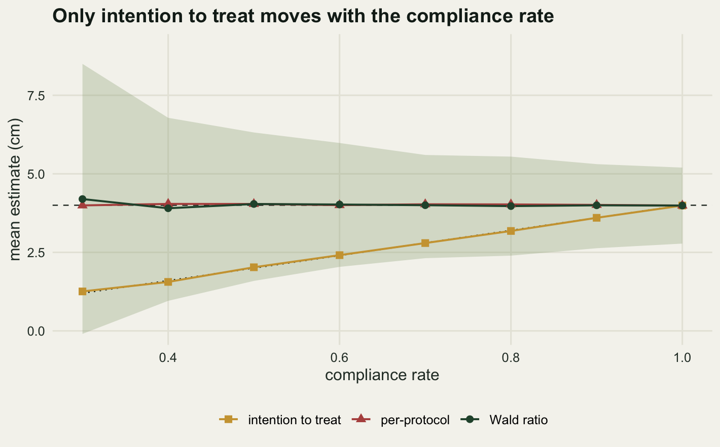
The intention-to-treat column tracks the closed form to 0.0561 centimetres at worst and 0.0208 on average, against a Monte Carlo standard error of 0.0301 on each entry. The worst gap is 1.8648 Monte Carlo standard errors, which is what a maximum over eight independent entries looks like when the underlying error is zero. The attenuation is linear in the compliance rate with nothing left over: at a compliance rate of 0.5 the estimate is half the effect. This is the sense in which intention to treat is honest about non-compliance. It is guaranteed to be too small, by a factor you can look up in your own field notes.
Per-protocol and the Wald ratio both sit on the true effect across the whole range, because in this version the fences that failed were a random subset. That is the situation the next section removes.
The Wald estimate is not free of small-sample trouble. At a compliance rate of 0.3 its mean over 1000 trials is 4.1971, which is 0.1971 above the truth: dividing by an estimated proportion makes this a ratio estimator, and a ratio estimator carries a small-sample bias that grows as its denominator shrinks. The spread matters more than the bias here. The standard deviation of the Wald estimate across trials is 3.2964 at a compliance rate of 0.3 and 0.9465 at full compliance, a factor of 3.4827, which is close to the factor of 3.3333 that one over the compliance rate predicts.
Per-protocol can change the sign of the answer
Random failure is the polite case. Fences do not fail at random: they fail where the ground is soft, and soft ground is wet ground, and wet ground grows a taller sward. That single sentence is enough to break the per-protocol comparison, because the set of plots with a standing fence is now a selected set, chosen by the same variable that drives the outcome.
The simulation makes compliance a logistic function of soil moisture, with slope g_comp controlling how strongly the two are tied. To keep the sweep clean, the intercept is solved at each step so that the average compliance rate stays at 0.6 whatever the slope is, which means the only thing changing along the sweep is the correlation between compliance and plot quality.
a_for <- function(g, target = 0.6) {
  f <- function(a) {
    integrate(function(q) plogis(a - g * q) * dnorm(q), -8, 8)$value - target
  }
  uniroot(f, c(-10, 10), tol = 1e-10)$root
}

set.seed(20260803)
g_grid <- seq(0, 3, length.out = 13)
n_rep_g <- 500

sweep_g <- t(vapply(g_grid, function(g) {
  a <- a_for(g)
  rowMeans(replicate(n_rep_g, {
    s <- sim_field(n_plot, a_comp = a, g_comp = g)
    c(three_est(s),
      rho = cor(s$q[s$z == 1], s$b[s$z == 1]),
      q_gap = mean(s$q[s$d == 1]) - mean(s$q[s$d == 0]))
  }))
}, numeric(6)))
sweep_g <- data.frame(slope = g_grid, sweep_g)

print(round(sweep_g[, c("slope", "rho", "comp", "itt", "pp", "late")], 4))
slope rho comp itt pp late
1 0.00 0.0020 0.5982 2.4063 4.0282 4.0259
2 0.25 -0.1156 0.6010 2.3850 2.9128 3.9649
3 0.50 -0.2309 0.6014 2.3965 1.8521 3.9864
4 0.75 -0.3267 0.6010 2.4189 0.9669 4.0530
5 1.00 -0.4082 0.5993 2.4716 0.2076 4.1428
6 1.25 -0.4738 0.5991 2.4105 -0.4396 4.0594
7 1.50 -0.5215 0.6009 2.4139 -0.8345 4.0448
8 1.75 -0.5644 0.5997 2.4270 -1.2299 4.0809
9 2.00 -0.5984 0.6014 2.3809 -1.5825 3.9928
10 2.25 -0.6257 0.6018 2.3668 -1.8489 3.9652
11 2.50 -0.6500 0.5978 2.3741 -2.0786 4.0140
12 2.75 -0.6650 0.6001 2.3983 -2.2426 4.0288
13 3.00 -0.6780 0.6009 2.4634 -2.2043 4.1420print(round(sweep_g[, c("slope", "q_gap", "pp")], 4)) slope q_gap pp
1 0.00 0.0027 4.0282
2 0.25 -0.1359 2.9128
3 0.50 -0.2685 1.8521
4 0.75 -0.3804 0.9669
5 1.00 -0.4702 0.2076
6 1.25 -0.5580 -0.4396
7 1.50 -0.6052 -0.8345
8 1.75 -0.6549 -1.2299
9 2.00 -0.6982 -1.5825
10 2.25 -0.7323 -1.8489
11 2.50 -0.7619 -2.0786
12 2.75 -0.7785 -2.2426
13 3.00 -0.7808 -2.2043mono <- sweep_g[sweep_g$slope <= 2, ]
cross_slope <- approx(mono$pp, mono$slope, xout = 0)$y
cross_rho <- approx(mono$pp, mono$rho, xout = 0)$y
pp_worst <- min(sweep_g$pp)
gap_worst <- sweep_g$q_gap[which.min(sweep_g$pp)]
print(round(c(crossing_slope = cross_slope, crossing_rho = cross_rho,
pp_at_zero_slope = sweep_g$pp[1],
pp_worst = pp_worst,
pp_error_worst = pp_worst - tau_true,
itt_range = diff(range(sweep_g$itt)),
late_range = diff(range(sweep_g$late))), 4)) crossing_slope crossing_rho pp_at_zero_slope pp_worst
1.0802 -0.4292 4.0282 -2.2426
pp_error_worst itt_range late_range
-6.2426 0.1047 0.1779 print(round(c(moisture_gap_at_worst = gap_worst,
gap_times_coefficient = 8 * gap_worst,
per_protocol_error = pp_worst - tau_true), 4))moisture_gap_at_worst gap_times_coefficient per_protocol_error
-0.7785 -6.2283 -6.2426 flip_long <- data.frame(
rho = rep(sweep_g$rho, 3),
value = c(sweep_g$itt, sweep_g$pp, sweep_g$late),
estimator = factor(rep(lab_e, each = nrow(sweep_g)), levels = lab_e))
ggplot(flip_long, aes(rho, value, colour = estimator, shape = estimator)) +
geom_hline(yintercept = 0, linetype = "dashed", colour = te_pal$ink,
linewidth = 0.4) +
geom_line(linewidth = 0.7) +
geom_point(size = 2.3) +
annotate("point", x = cross_rho, y = 0, size = 4.2, shape = 21,
colour = te_pal$clay, fill = NA, stroke = 1.1) +
scale_x_reverse() +
scale_colour_manual(values = c(te_pal$gold, te_pal$clay, te_pal$forest),
name = NULL) +
scale_shape_manual(values = c(15, 17, 16), name = NULL) +
labs(x = "correlation between compliance and soil moisture",
y = "mean estimate (cm)",
title = "Per-protocol crosses zero while the other two hold still") +
theme_te() +
theme(legend.position = "bottom")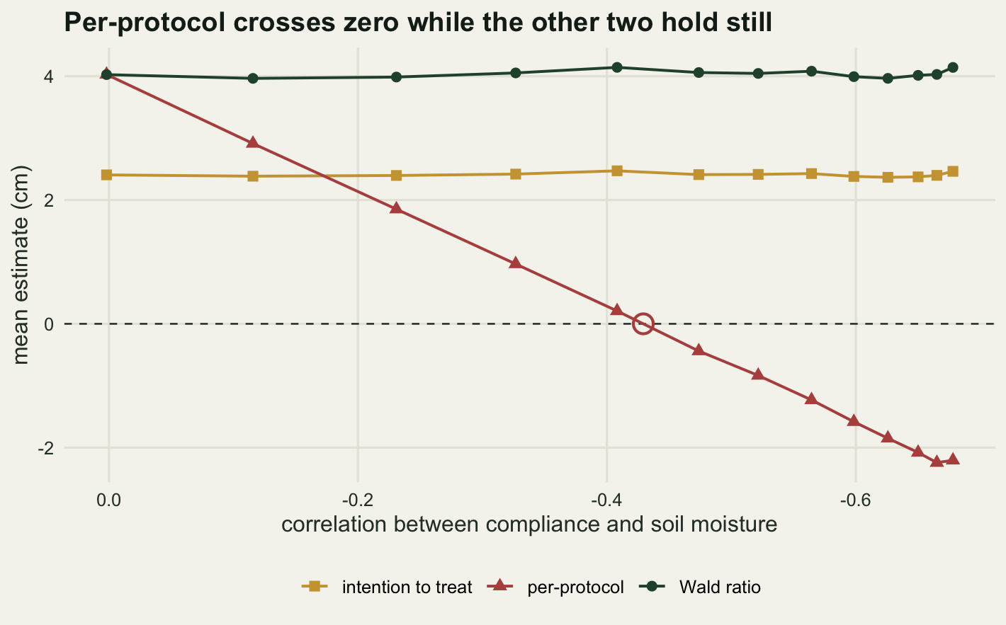
At the left edge, where compliance is unrelated to moisture, per-protocol returns 4.0282 and is the best of the three. Near the right edge it bottoms out at -2.2426, an error of -6.2426 centimetres on an effect of 4. The sign changes at a correlation of -0.4292 between compliance and soil moisture, which is a correlation an ecologist would describe as moderate and would not necessarily notice.
That is the substantive point of the post. A moderate association between whether the treatment stuck and how good the plot was is enough to make the per-protocol analysis report that exclosures reduce sward height when in fact every plot in the simulation would gain 4 centimetres from a working fence. The estimator is not merely attenuated; it is pointing the other way, and it does so with a standard error that looks respectable, because the plots really are different from each other.
Meanwhile the intention-to-treat estimate varies over a range of 0.1047 centimetres across the entire sweep and the Wald estimate over 0.1779. Neither notices. This is worth being precise about, because it is stronger than the usual statement. Selective compliance does not bias intention to treat at all. The derivation above never assumed that \(B_i\) was independent of \(Y_i(0)\): it only needed \(Z_i\) to be randomised, and \(Z_i\) was randomised by you. Selection into compliance moves which plots the effect is averaged over, and that is the subject of the next section, but it cannot contaminate the contrast itself.
The mechanism is visible in the covariate. The gap in mean soil moisture between the plots that ended up fenced and the rest runs from 0.0027 standard deviations at the left of the sweep to -0.7785 where per-protocol is at its worst. Multiplied by the moisture coefficient of 8 that gap is -6.2283 centimetres, against a per-protocol error of -6.2426. The estimator is reporting a moisture contrast with a treatment label on it.
The Wald ratio answers a question about the compliers
So far the effect has been the same 4 centimetres in every plot, which is why the Wald ratio came back with the right answer. Constant effects are a modelling convenience. In this system there is an obvious reason for the effect to vary: wetter plots grow faster and carry more grazing pressure, so keeping the cattle out of them does more. Let the effect be \(\tau_i = 4 + 3q_i\), so the average across the meadow is still 4 but a plot one standard deviation wetter gains 7 centimetres from a fence and a plot one standard deviation drier gains 1.
Now the two facts collide. Fences fail on wet plots, and wet plots are where fencing matters most. The plots that comply are the plots with the least to gain.
set.seed(20260806)
g_het <- 2
a_het <- a_for(g_het, 0.6)
tau_slope <- 3
big <- sim_field(2e5, tau0 = tau_true, tau1 = tau_slope,
                 a_comp = a_het, g_comp = g_het)

ate_true <- mean(big$tau_i)
late_true <- mean(big$tau_i[big$b == 1])
nonc_true <- mean(big$tau_i[big$b == 0])
q_comp <- mean(big$q[big$b == 1])
q_nonc <- mean(big$q[big$b == 0])

print(round(c(population_plots = length(big$q),
              compliance_rate = mean(big$b),
              ate = ate_true, late = late_true,
              non_complier_effect = nonc_true), 4))
population_plots compliance_rate ate late
2.0000e+05 6.0050e-01 4.0028e+00 2.5443e+00
non_complier_effect
6.1954e+00 print(round(c(late_minus_ate = late_true - ate_true,
percent_below_ate = 100 * (late_true - ate_true) / ate_true,
complier_minus_noncomplier = late_true - nonc_true,
mean_moisture_compliers = q_comp,
mean_moisture_failures = q_nonc), 4)) late_minus_ate percent_below_ate
-1.4585 -36.4367
complier_minus_noncomplier mean_moisture_compliers
-3.6511 -0.4852
mean_moisture_failures
0.7318 n_het <- 3000
het <- rowMeans(replicate(n_het, three_est(
sim_field(n_plot, tau0 = tau_true, tau1 = tau_slope,
a_comp = a_het, g_comp = g_het))))
print(round(c(mean_itt = het[["itt"]], mean_pp = het[["pp"]],
mean_wald = het[["late"]],
wald_minus_late = het[["late"]] - late_true,
itt_minus_pi_times_late =
het[["itt"]] - mean(big$b) * late_true,
itt_if_it_tracked_ate = mean(big$b) * ate_true), 4)) mean_itt mean_pp mean_wald
1.5038 -3.0474 2.5382
wald_minus_late itt_minus_pi_times_late itt_if_it_tracked_ate
-0.0061 -0.0241 2.4038 idx <- sample(seq_along(big$q), 40000)
dens_of <- function(keep, lab) {
dd <- density(big$tau_i[idx][keep], n = 512)
data.frame(x = dd$x, y = dd$y, group = lab)
}
keep_c <- big$b[idx] == 1
dens_dat <- rbind(dens_of(keep_c, "fence would hold (compliers)"),
dens_of(!keep_c, "fence would fail"))
dens_dat$group <- factor(dens_dat$group,
levels = c("fence would hold (compliers)",
"fence would fail"))
ggplot(dens_dat, aes(x, y, colour = group, fill = group)) +
geom_area(position = "identity", alpha = 0.35, colour = NA) +
geom_line(linewidth = 0.8) +
geom_vline(xintercept = ate_true, colour = te_pal$ink, linewidth = 0.6) +
geom_vline(xintercept = late_true, colour = te_pal$forest,
linetype = "dashed", linewidth = 0.6) +
annotate("text", x = ate_true + 0.3, y = 0.198, hjust = 0, size = 3.3,
colour = te_pal$ink, label = "average over all plots") +
annotate("text", x = late_true - 0.3, y = 0.198, hjust = 1, size = 3.3,
colour = te_pal$forest, label = "complier average") +
expand_limits(y = 0.21) +
scale_colour_manual(values = c(te_pal$forest, te_pal$clay), name = NULL) +
scale_fill_manual(values = c(te_pal$forest, te_pal$clay), name = NULL) +
labs(x = "true effect of a working exclosure (cm)", y = "density",
title = "The compliers are the plots with the least to gain") +
theme_te() +
theme(legend.position = "bottom")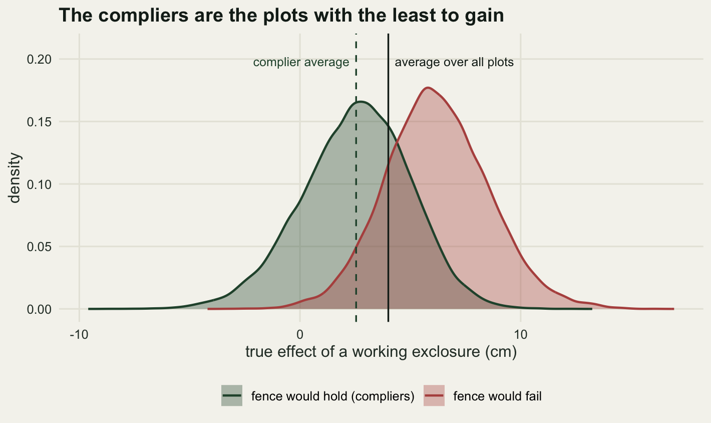
Averaged over the whole meadow the effect of a working exclosure is 4.0028 centimetres, which is what the simulation was told to do. Averaged over the plots whose fence would hold it is 2.5443. Averaged over the plots whose fence would fail it is 6.1954. The mean soil moisture of the two groups is -0.4852 and 0.7318 standard deviations, which is where the difference comes from.
The Wald ratio over 3000 simulated trials averages 2.5382, missing the complier average by -0.0061 and sitting 1.4585 centimetres below the average over all plots, which is 36.4367 per cent of it. The estimator did nothing wrong. It estimated the local average treatment effect, which is what Imbens and Angrist (1994) named it and what Angrist, Imbens and Rubin (1996) set out the conditions for, and the local part is not decoration. The trial has no information about the plots that lost their fences, because it never observed a working fence on any of them.
The same arithmetic explains the intention-to-treat number. It averages 1.5038, which is the compliance rate times the complier effect, 1.528, and not the compliance rate times the average effect over all plots, 2.4038. Both factors in that product moved.
The reporting consequence is concrete. If the paper says “fencing raised sward height by 2.54 centimetres”, the sentence is true of one subpopulation and false of the meadow, and the subpopulation is defined by something that was not measured directly: whether the fence would have held. Naming it costs one clause. What the trial estimates is the effect among plots where the exclosure survived the season, which here are the drier plots, and the effect on the wetter plots is larger and unmeasured. That clause also tells a reader why a scheme rolled out everywhere might do better than the trial suggested, or worse, depending on which way the selection ran.
There is one more case to note before leaving the ratio. If control plots can also pick up the treatment, the denominator is no longer a single compliance rate but the difference in receipt rates between the arms.
set.seed(20260807)
rate_treated_arm <- 0.7
rate_control_arm <- 0.15

sim_two_sided <- function(n, c1, c0, tau = tau_true) {
  q <- rnorm(n)
  z <- sample(rep(0:1, each = n / 2))
  d <- rbinom(n, 1, ifelse(z == 1, c1, c0))
  y <- 30 + 8 * q + tau * d + rnorm(n, 0, 5)
  itt <- mean(y[z == 1]) - mean(y[z == 0])
  denom <- mean(d[z == 1]) - mean(d[z == 0])
  c(itt = itt, denom = denom, wald = itt / denom)
}
n_ts <- 3000
ts <- rowMeans(replicate(n_ts, sim_two_sided(n_plot, rate_treated_arm,
                                             rate_control_arm)))
print(round(c(receipt_rate_treated_arm = rate_treated_arm,
              receipt_rate_control_arm = rate_control_arm,
              mean_itt = ts[["itt"]], mean_denominator = ts[["denom"]],
              mean_wald = ts[["wald"]], true_effect = tau_true), 4))
receipt_rate_treated_arm receipt_rate_control_arm mean_itt
0.7000 0.1500 2.1993
mean_denominator mean_wald true_effect
0.5508 3.9921 4.0000 With a receipt rate of 0.7 in the assigned arm and 0.15 in the control arm, the denominator averages 0.5508 and the Wald ratio averages 3.9921 against a true 4. The estimator still works, and it now needs an assumption it did not need before: no plot is fenced because it was assigned to control and unfenced because it was assigned to treatment. Defiers of that kind are rare in ecology but not unimaginable, since a contrary landowner is a real thing.
Compliance is a sample size problem before it is an estimation problem
A design that expects some non-compliance needs to be sized for it, and the sizing is where the intuition most often goes wrong. The intention-to-treat effect is \(\pi\tau\) and the standard error of a two-group mean difference with \(n\) plots split evenly is \(2\sigma/\sqrt{n}\), so the sample size for power \(1-\beta\) at level \(\alpha\) is
\[n = \frac{4\sigma^{2}(z_{1-\alpha/2} + z_{1-\beta})^{2}}{(\pi\tau)^{2}}\]
and the compliance rate enters squared. Seventy per cent compliance does not cost thirty per cent of the design. It costs a factor of \(1/0.7^2\), which is a little over two.
The sweep below computes that closed form and then ignores it, searching for the sample size that actually delivers 80 per cent power by simulation at each compliance rate.
set.seed(20260808)
pow_at <- function(n, cc, nsim, tau = tau_true, beta_q = 8, sigma = 5) {
  half <- n / 2
  z <- rep(0:1, each = half)
  crit <- qnorm(0.975)
  mean(replicate(nsim, {
    q <- rnorm(n)
    y <- 30 + beta_q * q + tau * z * rbinom(n, 1, cc) + rnorm(n, 0, sigma)
    y1 <- y[z == 1]
    y0 <- y[z == 0]
    abs(mean(y1) - mean(y0)) /
      sqrt(var(y1) / half + var(y0) / half) > crit
  }))
}

z_sum <- qnorm(0.975) + qnorm(0.8)
var_tot <- 8^2 + 5^2
n_closed <- function(cc) 4 * var_tot * z_sum^2 / (cc * tau_true)^2

c_pow <- c(0.4, 0.5, 0.6, 0.7, 0.85, 1)
pw <- t(vapply(c_pow, function(cc) {
  n_a <- n_closed(cc)
  n_try <- 2 * round(n_a * c(0.55, 0.75, 0.9, 1.05, 1.25, 1.5) / 2)
  p_try <- vapply(n_try, pow_at, numeric(1), cc = cc, nsim = 1200)
  c(n_closed = n_a, n_simulated = approx(p_try, n_try, xout = 0.8)$y,
    power_at_closed = pow_at(2 * round(n_a / 2), cc, 2000))
}, numeric(3)))
pw <- data.frame(compliance = c_pow, pw)
pw$ratio <- pw$n_simulated / pw$n_closed
pw$extra_vs_full <- pw$n_simulated / pw$n_simulated[nrow(pw)]

print(round(pw[, c("compliance", "n_closed", "n_simulated",
                   "power_at_closed", "ratio", "extra_vs_full")], 3))
compliance n_closed n_simulated power_at_closed ratio extra_vs_full
1 0.40 1091.485 1181.592 0.792 1.083 6.709
2 0.50 698.550 731.644 0.797 1.047 4.154
3 0.60 485.104 499.275 0.782 1.029 2.835
4 0.70 356.403 369.846 0.782 1.038 2.100
5 0.85 241.713 247.408 0.808 1.024 1.405
6 1.00 174.638 176.112 0.794 1.008 1.000slope_pw <- unname(coef(lm(log(n_simulated) ~ log(compliance),
data = pw))[2])
print(round(c(fitted_log_log_slope = slope_pw,
closed_form_slope = -2,
plots_at_full_compliance = pw$n_simulated[6],
plots_at_70_percent = pw$n_simulated[4],
multiplier_at_70 = pw$extra_vs_full[4],
one_over_c_squared_at_70 = 1 / 0.7^2), 4)) fitted_log_log_slope closed_form_slope plots_at_full_compliance
-2.0668 -2.0000 176.1124
plots_at_70_percent multiplier_at_70 one_over_c_squared_at_70
369.8462 2.1001 2.0408 c_fine <- seq(0.38, 1.02, length.out = 120)
curves <- rbind(
data.frame(compliance = c_fine, n = n_closed(c_fine),
rule = "closed form, one over compliance squared"),
data.frame(compliance = c_fine,
n = pw$n_closed[6] / c_fine,
rule = "one over compliance"))
ggplot(curves, aes(compliance, n, colour = rule, linetype = rule)) +
geom_line(linewidth = 0.8) +
geom_point(data = pw, inherit.aes = FALSE,
aes(compliance, n_simulated), colour = te_pal$gold,
size = 2.8, shape = 15) +
scale_x_log10(breaks = c(0.4, 0.5, 0.6, 0.7, 0.85, 1)) +
scale_y_log10(breaks = c(150, 250, 400, 700, 1200)) +
scale_colour_manual(values = c(te_pal$forest, te_pal$clay), name = NULL) +
scale_linetype_manual(values = c("solid", "22"), name = NULL) +
guides(colour = guide_legend(nrow = 2), linetype = guide_legend(nrow = 2)) +
labs(x = "compliance rate", y = "plots needed for 80 per cent power",
title = "The cost of non-compliance is quadratic") +
theme_te() +
theme(legend.position = "bottom")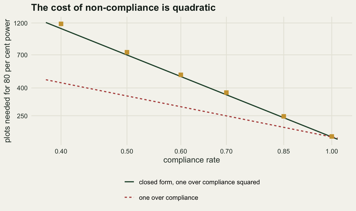
Fitting a line through the logarithms gives a slope of -2.0668 against the closed form’s exact minus two, so the quadratic rule is what the simulation finds. In plots: 176 at full compliance, 370 at seventy per cent, a multiplier of 2.1001 where one over the compliance rate would have predicted 1.4286 and one over its square predicts 2.0408. At forty per cent compliance the same effect needs 1182 plots, 6.7093 times the full-compliance design.
The closed form is slightly optimistic, and it is worth knowing by how much. The simulated requirement is between 1.0084 and 1.0826 times the formula, and the empirical power at the formula’s sample size comes out at 0.782 to 0.808, scattered around 0.8 rather than landing on it. The reason is that partial compliance adds variance to the assigned-treated arm that full compliance does not: within that arm, some plots got 4 centimetres and some got nothing, which contributes \(\tau^2\pi(1-\pi)\) to its variance. The formula above uses one common \(\sigma^2\) and misses it. The correction is small next to the factor the compliance rate itself contributes, but it means a power calculation done this way should be treated as a floor.
This is the number to put in front of whoever is deciding how many plots to fence. Spending on fence quality, or on a design that puts the exclosures where they can be maintained, buys sample size at a quadratic rate, and it is usually cheaper than the plots.
What you can check, and what you cannot
Everything above depended on the received-treatment column existing. Two diagnostics come with it, and neither is expensive.
The first is the compliance rate itself, with an interval, reported next to the effect. It is the denominator of the Wald ratio and the multiplier on the sample size, and a reader cannot reconstruct either without it.
The second is the balance check the sign flip section was crying out for: within the assigned-treated arm only, compare the plots that complied against the plots that did not, on every covariate you have. Randomisation says nothing about that comparison, because compliance was not randomised, so any difference is real and is exactly the thing that breaks per-protocol.
set.seed(20260809)
n_bal <- 1000
balance_p <- replicate(n_bal, {
  s <- sim_field(n_plot, a_comp = a_for(cross_slope), g_comp = cross_slope)
  arm <- s$z == 1
  t.test(s$q[arm & s$b == 1], s$q[arm & s$b == 0])$p.value
})
det_rate <- mean(balance_p < 0.05)

set.seed(20260810)
cover_naive <- function(n, cc = comp_rate, tau = tau_true) {
  half <- n / 2
  z <- rep(0:1, each = half)
  q <- rnorm(n)
  y <- 30 + 8 * q + tau * z * rbinom(n, 1, cc) + rnorm(n, 0, 5)
  y1 <- y[z == 1]
  y0 <- y[z == 0]
  e <- mean(y1) - mean(y0)
  s <- sqrt(var(y1) / half + var(y0) / half)
  c(covers_tau = abs(e - tau) < qnorm(0.975) * s,
    covers_itt = abs(e - cc * tau) < qnorm(0.975) * s)
}
n_cov <- c(n_plot, 4 * n_plot, 16 * n_plot)
cv <- t(vapply(n_cov, function(nn)
  rowMeans(replicate(1500, cover_naive(nn))), numeric(2)))
cv <- data.frame(plots = n_cov, cv)

set.seed(20260811)
var_hits <- replicate(2000, {
  s <- sim_field(n_plot, a_comp = qlogis(comp_rate))
  var.test(s$y[s$z == 1], s$y[s$z == 0])$p.value < 0.05
})
var_power <- mean(var_hits)

print(round(c(balance_test_slope = cross_slope,
              detection_rate_at_5pct = det_rate), 4))
balance_test_slope detection_rate_at_5pct
1.0802 1.0000 print(signif(c(median_p_value = median(balance_p),
largest_p_value = max(balance_p)), 3)) median_p_value largest_p_value
2.85e-10 6.04e-04 print(round(cv, 4)) plots covers_tau covers_itt
1 400 0.6013 0.9507
2 1600 0.0853 0.9413
3 6400 0.0000 0.9453print(round(c(coverage_drop = cv$covers_tau[1] - cv$covers_tau[3],
itt_coverage_range = diff(range(cv$covers_itt))), 4)) coverage_drop itt_coverage_range
0.6013 0.0093 print(round(c(extra_variance_in_treated_arm =
tau_true^2 * comp_rate * (1 - comp_rate),
total_variance = var_tot,
variance_ratio = 1 + tau_true^2 * comp_rate *
(1 - comp_rate) / var_tot,
var_test_detection_rate = var_power), 4))extra_variance_in_treated_arm total_variance
3.8400 89.0000
variance_ratio var_test_detection_rate
1.0431 0.0610 At the compliance-moisture slope where per-protocol crosses zero, a two-sample test of soil moisture between compliers and failures inside the treated arm has a p-value below 0.05 in 100 per cent of simulated trials, with a median p-value of 2.85e-10 and a largest p-value across 1000 trials of 6.04e-04. The check that would have caught the sign flip is a one-line t.test and it did not miss once.
Now the case where the column does not exist. Suppose nobody walked the fences, or the walk happened and was not written down. The analysis then has z and y and nothing else, and the intention-to-treat estimate is the only thing available. It is a perfectly good estimate of the effect of assignment. The trouble is that it will be read as the effect of fencing, and the second table shows what that costs.
The naive interval covers the intention-to-treat quantity 0.9507 of the time at 400 plots and 0.9453 at 6400, which is nominal at every size. Its coverage of the actual treatment effect is 0.6013 at 400 plots, 0.0853 at 1600, and 0 at 6400. Collecting more data makes it worse, which is the signature of a bias rather than noise: the interval shrinks around a point that is 1.6 centimetres away and eventually excludes the truth every time.
Nothing in the diagnostic output of that analysis complains. The residuals are fine, the randomisation check on the covariates passes because assignment really was random, the model is correctly specified for the data it was given. The only trace non-compliance leaves is the extra variance it puts in the assigned-treated arm, which for these parameters is \(\tau^2\pi(1-\pi) =\) 3.84 against a total variance of 89, a ratio of 1.0431. An F test comparing the two arms’ variances picks that up in 6.1 per cent of trials at 400 plots, against the 5 per cent it would fire at by chance, so it is a trace and not a diagnostic. If receipt is not recorded, non-compliance is not in the data at all, and the estimate is quietly attenuated by a factor nobody can name.
That is the practical instruction and it is a field-notebook instruction rather than a statistical one. Record what actually happened to each plot, at the plot level, at the end of the season. It converts an unknowable attenuation into a known one.
What to take away
Three estimators, one dataset, and they answer different questions. Intention to treat converges to the compliance rate times the effect among compliers, which the sweep confirmed to 0.0561 centimetres across compliance rates from 0.3 to 1. It is attenuated on purpose and by a known factor, and selective compliance does not touch it: over a sweep that dragged per-protocol from 4 to -2.2426, the intention-to-treat mean moved by 0.1047 centimetres in total.
Per-protocol is the one to avoid. When compliance was random it was fine; when compliance correlated with soil moisture at -0.4292 it reported zero effect, and at its worst it reported -2.2426 centimetres, the wrong sign on an effect of 4 present in every plot. The mechanism is that at that point the plots which kept their fences differed from the rest by -0.7785 standard deviations of soil moisture, and eight centimetres per standard deviation of moisture is enough to swamp a four-centimetre treatment.
The Wald ratio is unbiased for something, and the something has a name. With the effect varying across the meadow it returned 2.5382 against a complier average of 2.5443 and an all-plot average of 4.0028: 36.4367 per cent below the number a reader will assume it is. The plots that lost their fences had an average effect of 6.1954, and the trial contains no information about them.
And compliance is a design parameter with a quadratic price. The simulated sample size fell with the compliance rate at a fitted exponent of -2.0668, so seventy per cent compliance needs 2.1001 times the plots and forty per cent needs 6.7093 times.
The honest limit is where the whole apparatus rests. Every number in this post came from knowing which plots received the treatment, and the Wald ratio needs that column even more than the others do, because the column is its denominator. Without it, the analysis is not wrong, it is attenuated by an unknown factor between zero and one, and the coverage table is the demonstration: at 6400 plots the interval covered the true effect 0 of the time while looking exactly like an interval that covers 0.9453 of the time. There is a second limit the simulation cannot see past either. The derivation assumed a plot responds only to its own treatment, and an exclosure that concentrates grazing onto its unfenced neighbours breaks that assumption before any of this arithmetic starts: see interference between experimental plots for what that does.
References
Angrist JD, Imbens GW, Rubin DB 1996 Journal of the American Statistical Association 91(434):444-455 (10.1080/01621459.1996.10476902)
Imbens GW, Angrist JD 1994 Econometrica 62(2):467-475 (10.2307/2951620)
Bloom HS 1984 Evaluation Review 8(2):225-246 (10.1177/0193841X8400800205)
Kimmel K, Dee LE, Avolio ML, Ferraro PJ 2021 Trends in Ecology and Evolution 36(12):1141-1152 (10.1016/j.tree.2021.08.008)
Christie AP, Amano T, Martin PA, Shackelford GE, Simmons BI, Sutherland WJ 2019 Journal of Applied Ecology 56(12):2742-2754 (10.1111/1365-2664.13499)
Baylis K, Honey-Roses J, Borner J, Corbera E, Ezzine-de-Blas D, Ferraro PJ, Lapeyre R, Persson UM, Pfaff A, Wunder S 2016 Conservation Letters 9(1):58-64 (10.1111/conl.12180)
Ferraro PJ, Pattanayak SK 2006 PLoS Biology 4(4):e105 (10.1371/journal.pbio.0040105)
Gerber AS, Green DP 2012 Field Experiments: Design, Analysis, and Interpretation (ISBN 978-0-393-97995-4)
Hernan MA, Robins JM 2020 Causal Inference: What If (ISBN 978-1-4200-7616-5)