make_groups <- function(p, r, n_grp, n) {
  s <- sqrt(r); founder <- rbinom(n_grp, 1, p)
  copy <- runif(n_grp * n) < s                        # copy the founder, or draw afresh
  g <- ifelse(copy, rep(founder, each = n), rbinom(n_grp * n, 1, p))
  grp <- rep(seq_len(n_grp), each = n)
  list(g = g, grp = grp, go = (ave(g, grp, FUN = sum) - g) / (n - 1), n = n)
}
pcov <- function(x, y) mean((x - mean(x)) * (y - mean(y)))   # population covariance
sel  <- function(g, w) pcov(w / mean(w), g)                    # selection on the allele
# the three regressions of Hamilton's rule, and the identity that ties them to selection
hamilton_parts <- function(g, go, w) {
  co <- coef(lm(w ~ g + go))
  out <- c(S = sel(g, w), r = pcov(go, g) / pcov(g, g), b = unname(co["go"]),
           c = -unname(co["g"]), V = pcov(g, g), wbar = mean(w))
  stopifnot(abs(out[["S"]] * out[["wbar"]] -
                out[["V"]] * (out[["b"]] * out[["r"]] - out[["c"]])) < 1e-10)
  out
}
n_grp <- 12000; n <- 4; r0 <- 0.5; c0 <- 1; p0 <- 0.3
set.seed(1414)
pop <- make_groups(p0, r0, n_grp, n)
payoff <- function(pop, b, c = c0, d = 0) 1 - c * pop$g + b * pop$go + d * pop$g * pop$go14 Checking a kin selection analysis
Chapter 13 ended with Hamilton’s rule rewritten as a statement about regression coefficients. Selection on a social allele is the covariance between fitness and genotype; regress fitness on an individual’s own genotype and on the genotype of its social partners, call the first slope minus the cost and the second the benefit, take relatedness to be the regression of the partners’ genotype on the individual’s own, and rb - c then has the sign of selection by construction. In that form the rule cannot fail. It is an accounting identity in the same sense as the Price equation of Chapter 12, and it holds in any population for which the three regressions can be computed. What can fail is the step every applied study takes before the rule is used: a cost, a benefit and a relatedness are measured separately, from an experiment, a field estimate and a pedigree, and multiplied together as if they were the three slopes. This chapter measures four ways in which those plug-in numbers differ from the slopes that selection actually uses, and in each case how far the verdict of the rule moves when they do.
14.1 A population of groups and the regression form
The simulated population is made of groups of relatives, the smallest structure in which kin selection can act. Each individual either carries an allele for helping or does not. Within a group, genotypes are correlated: each member copies a group founder with a fixed probability and otherwise draws a fresh allele from the population, which makes the correlation between any two groupmates equal to the square of the copying probability. The copying probability is therefore set to the square root of the relatedness asked for. An individual’s fitness depends on its own genotype g, through the cost of helping, and on \(g'\), the mean genotype of its groupmates, through the help it receives.
The function hamilton_parts() returns the selection differential on the allele, the regression relatedness, and the benefit and cost as partial regression slopes of absolute fitness, and it stops if the identity linking them fails. The identity is the one Chapter 13 proved for least squares slopes, and every call below passes it. The population has 12,000 groups of 4, an allele frequency of 0.30, a nominal relatedness of 0.50 among groupmates, the value for full siblings, and a cost of helping of 1.00 fitness units.
b_add <- 1.8
hp_add <- hamilton_parts(pop$g, pop$go, payoff(pop, b_add))
stopifnot(abs(hp_add[["b"]] - b_add) < 1e-8, abs(hp_add[["c"]] - c0) < 1e-8)
With additive payoffs and a benefit of 1.80, the regression recovers the plug-in values to the precision of the arithmetic: the benefit slope is 1.800 and the cost slope 1.000. The realised relatedness in this finite population is 0.498, and the selection differential is -0.017, negative, as rb - c of -0.10 says it should be. When fitness really is the sum of a cost and a benefit, the separately measured numbers and the slopes are the same thing. The four checks break that equality one assumption at a time.
14.2 Payoffs that do not add
Much cooperation pays more when the partner cooperates too. Two birds mobbing a predator drive it off where one would not; two workers lift a load that neither could move alone. A single term captures it: an individual that helps and has helping partners gains an extra d times the partners’ mean genotype, on top of the cost it pays and the benefit it receives.
d_syn <- 2
hp_syn <- hamilton_parts(pop$g, pop$go, payoff(pop, b_add, d = d_syn))
plug_syn <- r0 * b_add - c0
At the same benefit of 1.80 and a synergy of 2.00, the plug-in rule still gives rb - c of -0.10, since neither the cost nor the benefit was changed, and still predicts that helping is selected against. The allele is in fact favoured: the selection differential is 0.154, larger in magnitude than the negative value of the additive case. The regression form is not fooled. Its benefit slope is 2.693 and its cost slope 0.147, so the synergy has been split between them: part of it looks like a larger benefit, and part like a smaller cost, because a helper’s own help is repaid in proportion to how often its partners help as well. With these slopes rb - c is 1.195 and the rule gives the right sign.
The split is the difficulty. How much of the synergy lands in the benefit and how much in the cost depends on how often helpers meet helpers, which depends on the allele frequency. For binary genotypes in this population the selection differential works out as the variance of g times \(-c + br + d\,[p + r(1-p)]\), divided by mean fitness, and the bracket moves with p. An additive payoff has no such dependence on frequency; a synergistic one can change the sign of selection as the allele spreads.
b_f <- 0.8; d_f <- 0.8
p_grid <- seq(0.05, 0.95, by = 0.1)
set.seed(1415)
freq <- do.call(rbind, lapply(p_grid, function(p) {
  po <- make_groups(p, r0, n_grp, n)
  ha <- hamilton_parts(po$g, po$go, payoff(po, b_f))
  hs <- hamilton_parts(po$g, po$go, payoff(po, b_f, d = d_f))
  data.frame(p = p, S_add = ha[["S"]], S_syn = hs[["S"]], b_syn = hs[["b"]], c_syn = hs[["c"]])
}))
p_star <- ((c0 - b_f * r0) / d_f - r0) / (1 - r0)          # where the bracket changes sign
pred_S <- function(p, d) p * (1 - p) * (-c0 + b_f * r0 + d * (p + r0 * (1 - p))) /
  (1 + (b_f - c0) * p + d * p * (p + r0 * (1 - p)))
stopifnot(all(sign(freq$S_syn[abs(freq$p - p_star) > 0.1]) ==
              sign(freq$p[abs(freq$p - p_star) > 0.1] - p_star)))
lo <- 1; hi <- nrow(freq); i75 <- which.min(abs(freq$p - 0.75))
Take a benefit of 0.80 and a synergy of the same size. The plug-in rb - c is -0.60, and a study that took it at face value would conclude that helping is selected against at every frequency. It is selected against while the allele is rare: at a frequency of 0.05 the selection differential is -0.010, small only because a rare allele has little variance for selection to act on. The bracket changes sign at a frequency of 0.50, and above it selection favours helping, reaching 0.015 at a frequency of 0.75. The population has two stable states, one without helpers and one where every individual helps, and which it reaches depends on where it starts. The regression benefit rises from 1.085 at the lowest frequency to 1.299 at the highest, and the regression cost falls from 0.731 to 0.484, so the slopes that make the rule exact are properties of the current population and not of the behaviour. Chapter 13 met the opposite case, a benefit that saturates, in which selection holds the allele at an intermediate frequency; synergy turns that stable point into a threshold.
p_fine <- seq(0.02, 0.98, length.out = 200)
lines_df <- rbind(data.frame(p = p_fine, S = pred_S(p_fine, 0), payoff = "additive"),
                  data.frame(p = p_fine, S = pred_S(p_fine, d_f), payoff = "synergistic"))
pts_df <- rbind(data.frame(p = freq$p, S = freq$S_add, payoff = "additive"),
                data.frame(p = freq$p, S = freq$S_syn, payoff = "synergistic"))
ggplot(lines_df, aes(p, S, colour = payoff)) +
  geom_hline(yintercept = 0, colour = te_line) +
  geom_vline(xintercept = p_star, colour = te_sage, linetype = "dashed") +
  geom_line(linewidth = 0.8) +
  geom_point(data = pts_df, size = 2) +
  scale_colour_manual(values = c(additive = te_forest, synergistic = te_rust), name = NULL) +
  labs(x = "frequency of the helping allele", y = "selection on the allele") +
  theme_book()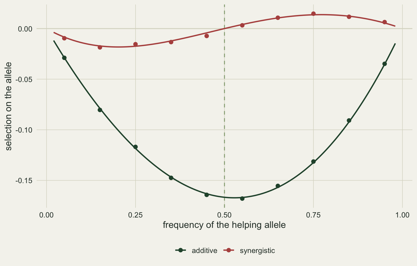
A single field estimate of the benefit of help is a measurement at one frequency. Under additive payoffs that is enough; under synergy it is the slope at that frequency only, and it cannot say whether the population sits on the side where helping spreads or the side where it is lost. The check is to ask whether the payoff to being helped depends on whether one helps oneself, which an experiment can measure by crossing the two, and if it does, to report the rule at the frequency where the answer is wanted.
14.3 Relatives who are also competitors
The second assumption is that raising the fitness of a relative is a gain. Fitness is relative, and if the helped relative competes for the same territories, mates or breeding sites as the helper and its other kin, part of what the help adds to the relative is taken from them. West and colleagues (2002) reviewed how competition between relatives can reduce or cancel the benefit of kin selection, and Queller (1994) gave the accounting that Chapter 13 applied to demes: relatedness has to be measured relative to the individuals one competes with.
In the simulation a share kappa of competition happens within the group. Each individual’s fitness is its absolute payoff minus kappa times the amount by which its group’s mean payoff exceeds the population baseline, so with kappa at zero the group’s productivity is exported and with kappa at one it is spent entirely on rivalry within the group.
b_comp <- 2.5
local_fit <- function(pop, b, a, c = c0) {
  wa <- payoff(pop, b, c); wa - a * (ave(wa, pop$grp) - 1)
}
a_grid <- seq(0, 1, by = 0.1)
comp <- data.frame(a = a_grid,
                   S = vapply(a_grid, function(a) sel(pop$g, local_fit(pop, b_comp, a)), 0))
R_grp <- (1 + (n - 1) * r0) / n                     # relatedness to a random groupmate, self included
pred_comp <- function(a) p0 * (1 - p0) * (-c0 + b_comp * r0 - a * (b_comp - c0) * R_grp) /
  (1 + (1 - a) * (b_comp - c0) * p0)
a_star <- (b_comp * r0 - c0) / ((b_comp - c0) * R_grp)
gap_comp <- pred_comp(a_grid) - comp$S
stopifnot(all(gap_comp > 0), diff(range(gap_comp)) < 0.1 * mean(gap_comp))
hp_loc <- hamilton_parts(pop$g, pop$go, local_fit(pop, b_comp, 1))
stopifnot(abs(hp_loc[["b"]] - hp_loc[["c"]]) < 1e-8,
          abs(hp_loc[["c"]] - ((n - 1) * c0 + b_comp) / n) < 1e-8)
r_local <- (r0 - R_grp) / (1 - R_grp)               # relatedness relative to local competitors
r_grid <- c(0.25, 0.5, 0.75, 0.95)
set.seed(1416)
S_r <- vapply(r_grid, function(r) {
  po <- make_groups(p0, r, n_grp, n); sel(po$g, local_fit(po, b_comp, 1))
}, 0)
With a benefit of 2.50 the plug-in rb - c is 0.25, and with competition that is global the allele spreads, with a selection differential of 0.036. The differential falls steadily as competition becomes local, changes sign, on the prediction line, when kappa reaches 0.267, and under entirely local competition is -0.145, more strongly against helping than the global case was for it. A little more than a quarter of competition taking place among groupmates is enough to cancel a benefit that the plug-in rule reads as comfortably sufficient.
ggplot(comp, aes(a, S)) +
  geom_hline(yintercept = 0, colour = te_line) +
  geom_vline(xintercept = a_star, colour = te_sage, linetype = "dashed") +
  geom_line(data = data.frame(a = a_grid, S = pred_comp(a_grid)), colour = te_forest, linewidth = 0.8) +
  geom_point(colour = te_rust, size = 2.2) +
  labs(x = "share of competition within the group", y = "selection on the allele") +
  theme_book()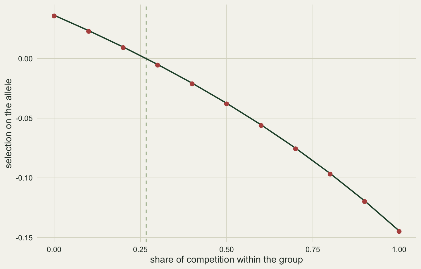
The measured points lie below the line by 0.0006 at every share, a small constant offset that comes from the line using the nominal relatedness while this finite population is slightly less related. The regression form again absorbs everything. Under full local competition its benefit and cost slopes are both 1.375, equal to the precision of the arithmetic, so helping a groupmate is repaid exactly by the competition it creates and any relatedness below one leaves rb - c negative. Measured against local competitors in Queller’s way, relatedness among these siblings is -0.333, below zero, and it takes that value at any pedigree relatedness, because against its own group an individual’s groupmates always deviate in the opposite direction to itself.
The natural rescue is to raise relatedness, since a more viscous population has more closely related groups. It does not work. Under full local competition the selection differential at relatedness 0.25, 0.50, 0.75 and 0.95 is -0.214, -0.146, -0.070 and -0.014. Higher relatedness reduces the variation within groups on which selection acts and so shrinks the differential towards zero, but it never turns it positive, because the individuals a helper aids and the individuals it competes with are the same individuals. A kin selection argument for a behaviour among neighbours therefore needs an estimate of the scale of competition, and a pedigree cannot supply it.
14.4 Help that does not reach relatives
The rule weighs the benefit by the relatedness between the helper and the individual actually helped. A study that records the relatedness within groups and the benefit of help assumes that the help goes to the groupmates. In the next simulation only a share q of each helper’s benefit is given to its own group; the rest is spread over the whole population, where the average recipient has the population’s genotype.
b_tgt <- 3
q_grid <- c(1, 0.75, 0.5, 0.25, 0)
target_fit <- function(pop, b, q, c = c0) 1 - c * pop$g + b * (q * pop$go + (1 - q) * mean(pop$g))
S_q <- vapply(q_grid, function(q) sel(pop$g, target_fit(pop, b_tgt, q)), 0)
q_star <- c0 / (r0 * b_tgt)
S_q0_pred <- -c0 * pcov(pop$g, pop$g) / mean(target_fit(pop, b_tgt, 0))
stopifnot(abs(S_q[length(S_q)] - S_q0_pred) < 1e-12)
hp_tgt <- hamilton_parts(pop$g, pop$go, target_fit(pop, b_tgt, 0.5))
At a benefit of 3.00 and full targeting, the plug-in rb - c is 0.50 and the allele is favoured, with a differential of 0.065. Because the benefit that leaves the group lands on a random recipient, the rule with correct inputs requires q times relatedness times benefit to exceed the cost, which puts the threshold at a targeting share of 0.667. The measured differentials agree: 0.016 at a share of 0.75, then -0.033 at 0.50. With no targeting at all the differential is -0.131, which is exactly the cost times the variance of g divided by mean fitness. Help given to everyone raises everyone’s fitness by the same amount, carries no covariance with the helper’s genotype, and leaves only the cost for selection to see.
The quantity that matters is the relatedness between actor and recipient, a fact about who interacts with whom. Relatedness measured within the social group describes the recipients only if the help stays in the group, and in a field study that has to be established by watching where the help goes.
14.5 Relatedness from a pedigree with wrong fathers
The last check returns to the pedigree. In the animal model of Chapter 7 relatedness entered as the off-diagonal of the relationship matrix A, a pedigree fraction of one half for full siblings, and Chapter 10 showed what happens to a heritability estimate when a share of the recorded fathers are wrong. A kin selection analysis that takes relatedness from the same pedigree inherits the same error, now in the relatedness that multiplies the benefit. In a songbird the social father feeds the whole brood, but some chicks were sired by other males, and chicks that share a mother but not a father are half siblings.
The simulation below is diploid. Each nest has a mother and a social father, drawn independently from a population at Hardy-Weinberg equilibrium; each chick takes one allele from its mother and one from its social father, except that with probability e its paternal allele comes from an unrelated extra-pair male. Alongside the helping locus every animal carries a set of neutral markers. Each chick helps its nestmates at a cost to itself, and g is now the frequency of the helping allele within the chick.
sim_nests <- function(n_nest, k, e, p, n_mark) {
  freqs <- c(p, runif(n_mark, 0.1, 0.9)); L <- length(freqs)
  gam <- function(m) matrix(rbinom(m * L, 1, rep(freqs, each = m)), m)   # one gamete per row
  dam1 <- gam(n_nest); dam2 <- gam(n_nest); sir1 <- gam(n_nest); sir2 <- gam(n_nest)
  N <- n_nest * k; nest <- rep(seq_len(n_nest), each = k)
  from_dam  <- ifelse(matrix(runif(N * L) < 0.5, N), dam1[nest, ], dam2[nest, ])
  from_sire <- ifelse(matrix(runif(N * L) < 0.5, N), sir1[nest, ], sir2[nest, ])
  ep <- runif(N) < e
  from_sire[ep, ] <- gam(sum(ep))                                        # extra-pair sire
  G <- (from_dam + from_sire) / 2
  list(g = G[, 1], mark = G[, -1, drop = FALSE], nest = nest)
}
others <- function(x, nest, k) (ave(x, nest, FUN = sum) - x) / (k - 1)
r_markers <- function(po, k) {                     # regression relatedness pooled over markers
  mo <- apply(po$mark, 2, others, nest = po$nest, k = k)
  sum(vapply(seq_len(ncol(po$mark)), function(j) pcov(mo[, j], po$mark[, j]), 0)) /
    sum(apply(po$mark, 2, function(x) pcov(x, x)))
}
n_nest <- 10000; k <- 4; b_ep <- 2.5; n_mark <- 40; r_ped <- 0.5
e_grid <- seq(0, 0.5, by = 0.1)
set.seed(1417)
ep_res <- do.call(rbind, lapply(e_grid, function(e) {
  po <- sim_nests(n_nest, k, e, p0, n_mark)
  go <- others(po$g, po$nest, k)
  w <- 1 - c0 * po$g + b_ep * go
  hp <- hamilton_parts(po$g, go, w)
  rm <- r_markers(po, k)
  data.frame(e = e, S = hp[["S"]], r_locus = hp[["r"]], r_mark = rm,
             S_ped = hp[["V"]] * (b_ep * r_ped - c0) / hp[["wbar"]],
             S_mark = hp[["V"]] * (b_ep * rm - c0) / hp[["wbar"]])
}))
r_expected <- function(e) 0.25 + 0.25 * (1 - e)^2    # half siblings through the mother, full through a shared sire
e_star <- 1 - sqrt(4 * c0 / b_ep - 1)                # extra-pair rate at which r b = c
i3 <- which(abs(e_grid - 0.3) < 1e-9)

# a study of realistic size: how precisely do markers place relatedness?
n_nest_s <- 150; n_mark_s <- 20; n_rep <- 300
set.seed(1418)
r_small <- replicate(n_rep, r_markers(sim_nests(n_nest_s, k, e_grid[i3], p0, n_mark_s), k))
With a benefit of 2.50 and the pedigree relatedness of 0.50, the plug-in rb - c is 0.25 at every rate of extra-pair paternity, since the pedigree records the social father whatever happened. The actual relatedness between nestmates is a quarter through the shared mother plus a quarter times the chance that both chicks were sired by the social father, and it falls below the c / b of 0.40 once the extra-pair rate exceeds 0.225. At a rate of 0.30, relatedness regressed at the helping locus is 0.378, the marker estimate is 0.373 and the expectation 0.372. The pedigree predicts a selection differential of 0.018, the markers predict -0.005, and the simulated differential is -0.004: the pedigree gets the sign wrong and the markers get it right.
ep_long <- rbind(data.frame(e = e_grid, S = ep_res$S_ped, series = "pedigree relatedness"),
                 data.frame(e = e_grid, S = ep_res$S_mark, series = "marker relatedness"))
ggplot(ep_long, aes(e, S, colour = series)) +
  geom_hline(yintercept = 0, colour = te_line) +
  geom_vline(xintercept = e_star, colour = te_sage, linetype = "dashed") +
  geom_line(linewidth = 0.8) +
  geom_point(data = transform(ep_res, series = "simulated"), aes(e, S), size = 2.2) +
  scale_colour_manual(values = c("pedigree relatedness" = te_gold, "marker relatedness" = te_forest,
                                 simulated = te_rust), name = NULL) +
  labs(x = "rate of extra-pair paternity", y = "selection on the allele") +
  theme_book()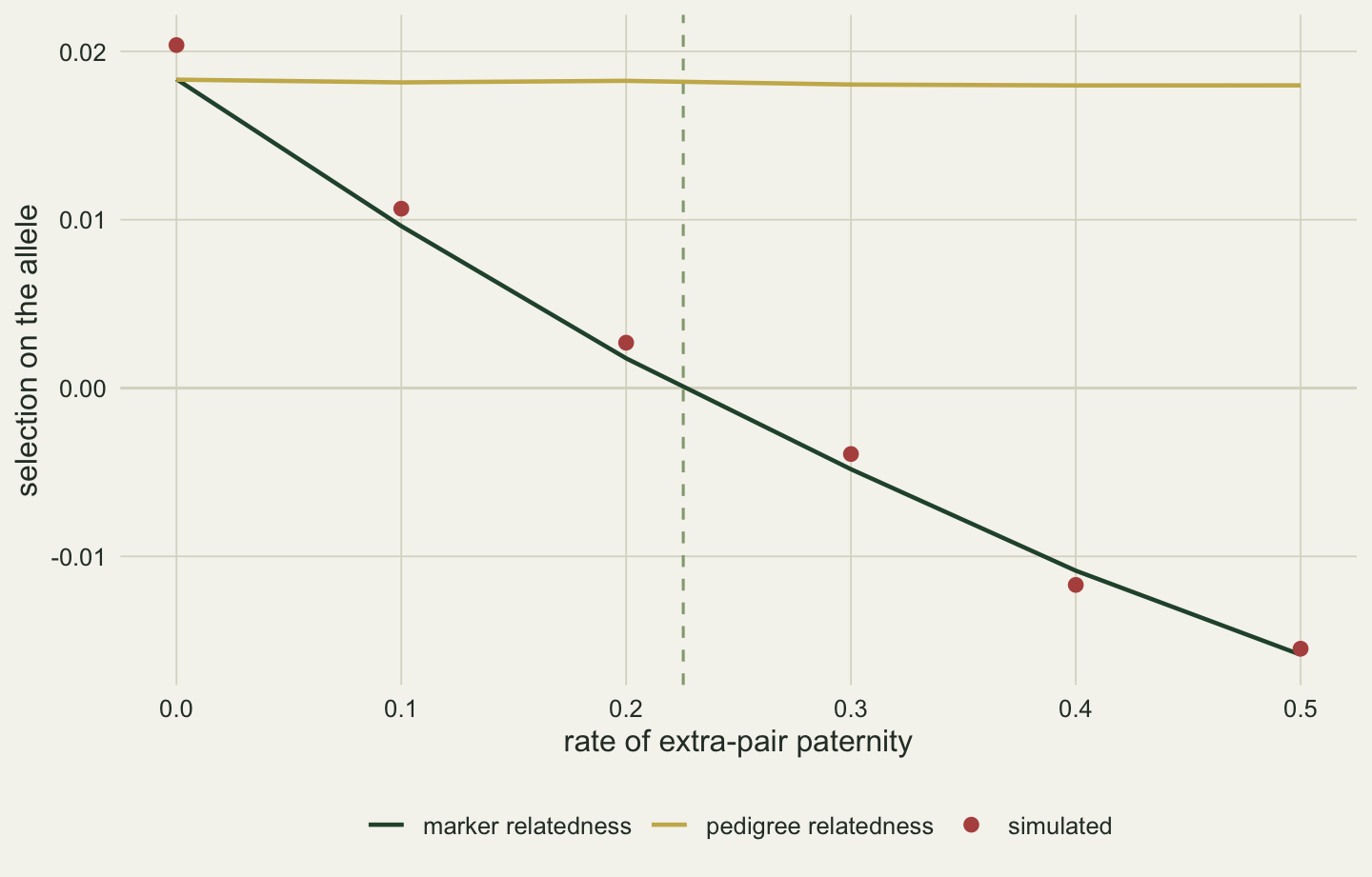
The marker estimate does not need a large study to settle the question. In 300 simulated studies of 150 nests with 20 markers at the same extra-pair rate, the pooled regression relatedness averaged 0.370 with a standard deviation of 0.012, and exceeded the threshold of 0.40 in 1.3 per cent of them. The sign problem that the pedigree creates is one that genotypes resolve cheaply, and it goes one step beyond the remedy Chapter 10 reached for the heritability, where genotyping a sample of broods estimated the extra-pair rate: here the genotypes measure the relatedness itself instead of inferring it from who was seen at the nest. Relatedness estimated this way is also the quantity the regression form asks for, a slope of partners’ genotype on one’s own, rather than a fraction read from a family tree.
14.6 What the checks have in common
In all four checks the regression form of the rule stayed exact, and in all four the plug-in version went wrong. The synergy was hidden in slopes that change with allele frequency, the competition in a benefit that is repaid at the helper’s expense, the untargeted help in a relatedness that described the wrong recipients, and the extra-pair young in a relatedness that described the wrong fathers. None of these failures shows in the rule itself. Each shows only when the cost, the benefit and the relatedness are defined against the population that actually interacts and competes, the definitions West, Griffin and Gardner (2007) argued social evolution needs if its terms are to mean anything. A kin selection analysis is checked by asking of each input whether it is that regression, and by measuring it as one where it is not.
This chapter closes the technical part of the book. Every chapter since the first has written selection or inheritance as a covariance or a regression and then checked what happens when the quantities in it are measured with error, against the wrong baseline or from the wrong relatives. The closing chapter draws those checks together and asks what a quantitative genetic analysis of a wild population can promise, and what it cannot.
References
West SA, Pen I, Griffin AS 2002. Science 296(5565):72-75 (10.1126/science.1065507)
Queller DC 1994. Evolutionary Ecology 8(1):70-73 (10.1007/BF01237667)
West SA, Griffin AS, Gardner A 2007. Journal of Evolutionary Biology 20(2):415-432 (10.1111/j.1420-9101.2006.01258.x)