set.seed(431)
n   <- 3000
rho <- 0.6
b2  <- 0.35
z2  <- rnorm(n)
z1  <- rho * z2 + sqrt(1 - rho^2) * rnorm(n)
W   <- rpois(n, exp(0.30 + b2 * z2))
w   <- W / mean(W)

shift1  <- sum(w * z1) / n - mean(z1)
covpop1 <- mean((z1 - mean(z1)) * (w - mean(w)))
stopifnot(abs(shift1 - covpop1) < 1e-12)

S1 <- cov(z1, w)
S2 <- cov(z2, w)
n_fac <- n / (n - 1)1 Selection as a covariance
A season of fieldwork on a marked population ends with two kinds of column. One kind holds the traits that were measured on every animal: body mass, wing length, laying date, a score from a behavioural test. The other holds a count of how well each animal did, in whatever currency the study could afford: offspring fledged, seeds set, whether it was seen alive the following spring. Everything in the first part of this book is about the relationship between those two kinds of column, and this chapter is about the simplest version of it.
The simplest version is already enough to go wrong. Traits are measured one at a time but they do not vary one at a time. Large birds tend to be in better condition, lay earlier and hold better territories, so if large birds leave more young, the data alone do not say whether size is being selected or is merely standing next to something that is. The chapter builds the two quantities that separate those readings, the selection differential and the selection gradient, and the identity that ties them together. It closes on what the gradient estimates when the fitness surface is not a flat plane, which is the case in every real population, and on the condition under which that estimate means what it is usually taken to mean.
1.1 Fitness, made relative
Absolute fitness W is whatever was counted. Relative fitness divides it by the population mean,
\[ w_i = \frac{W_i}{\bar W}, \]
so that the average individual has a relative fitness of exactly one. The division is not cosmetic. It turns fitness into a weight: an individual with relative fitness two contributes twice its share to the next generation, one with a half contributes half. The mean of a trait among the parents of the next generation, before any inheritance happens, is then the fitness-weighted mean of the trait,
\[ \bar z^{*} = \frac{1}{n} \sum_i w_i z_i , \]
and the change within the generation is that weighted mean minus the plain one. A line of algebra turns the difference into a covariance:
\[ S = \bar z^{*} - \bar z = \operatorname{cov}(z, w). \]
This is the selection differential. It is the whole of what selection did to the trait mean in one generation, measured before reproduction has any chance to copy it forward. Nothing in the derivation assumes normality, linearity or anything about genetics; it is the definition of a weighted mean rearranged.
Here is a population where the answer is known because the simulation sets it. Every animal carries two standardised traits, z1 and z2, correlated with each other. Offspring number is Poisson with a mean that rises with z2 and does not depend on z1 at all.
Among the 3,000 animals, the fitness-weighted mean of z1 sits 0.211 standard deviations above the plain mean, and the population covariance of z1 with relative fitness is the same number to the last floating-point digit. One practical detail belongs here because it causes needless confusion: cov() in R divides by n - 1, not by n, so it returns a differential larger by a factor of 1.0003. At any sample size worth analysing the difference is invisible, and every differential below uses cov().
Both traits have positive differentials, 0.211 for z1 and 0.352 for z2. The first of those numbers is the problem this chapter exists to solve. The simulation gave z1 no effect on fitness whatsoever, yet the animals that bred were, on average, larger on z1 than the animals that did not. The ratio of the two differentials is 0.599, close to the trait correlation of 0.60, and that is not a coincidence: all z1 receives is the selection on z2, passed through the correlation between them.
1.2 Units that can be compared
A differential is in the units of the trait. That is fine for one trait in one population and useless for anything else, because a differential of two grams on body mass and one of three days on laying date cannot be set side by side. The usual remedy, and the one used throughout this book, is to standardise every trait to a mean of zero and a variance of one before computing anything. The differential is then in phenotypic standard deviations, and it has a second reading: for a standardised trait, S is the covariance of the trait with relative fitness and also the correlation between them multiplied by the standard deviation of relative fitness. Selection on a trait can never exceed the variation in fitness that is there to do the selecting.
Variance standardisation has a cost that is worth knowing about before it is relied on. It makes a differential depend on how variable the trait happens to be in the sample: the same fitness function, applied to a population whose trait variance has been cut by a bottleneck or a harsh year, reads as weaker selection, because each standard deviation now spans fewer grams. Hereford and colleagues (2004) argued for standardising by the trait mean instead, which gives an elasticity: the proportional change in fitness per proportional change in the trait. Both conventions are defensible, they answer different questions, and a paper that does not say which it used cannot be compared with anything. The chapters that follow use variance-standardised traits and relative fitness, and say so whenever the choice matters.
1.3 Direct selection: the gradient
The way to separate the target from the passenger is to ask what happens to fitness when one trait changes and the others do not. With observational data nobody can hold a trait fixed, but a multiple regression does the equivalent arithmetic: each partial coefficient describes the change in expected relative fitness per unit of its trait, with the other traits in the model held constant. Lande and Arnold (1983) made that regression the standard measure of direct selection and called its coefficients the selection gradients, collected in a vector beta.
m_lin <- lm(w ~ z1 + z2)
beta  <- coef(m_lin)[c("z1", "z2")]
tab   <- summary(m_lin)$coefficients
The gradient on z2 is 0.350, standard error 0.019, against the 0.35 the simulation built in. The gradient on z1 is 0.001 with a p-value of 0.95: once z2 is in the model there is nothing left for z1 to explain. The regression has done what the differential could not, and put the selection on the trait that carried it.
That is the core distinction of the chapter, and it is worth stating plainly. The differential describes what happened to a trait. The gradient describes what acted on it. They are different quantities, both are useful, and a paper that reports one under the name of the other has misreported its result.
1.4 The identity that joins them
The two quantities are not separate measurements. Collect the differentials into a vector S and the phenotypic covariance matrix of the traits into P. The least squares gradient is then
\[ \boldsymbol\beta = \mathbf P^{-1} \mathbf S , \]
which is nothing more than the normal equations of the regression written in covariances. Multiple regression performs that inversion internally, so the two routes to beta agree.
P    <- cov(cbind(z1, z2))
S    <- c(S1, S2)
beta_P <- drop(solve(P) %*% S)
stopifnot(max(abs(beta_P - beta)) < 1e-10)

direct   <- diag(P) * beta_P
indirect <- S - direct
The matrix route and the regression agree to the precision of the arithmetic. Read backwards the identity says more than it does forwards:
\[ \mathbf S = \mathbf P \boldsymbol\beta , \qquad S_1 = P_{11} \beta_1 + P_{12} \beta_2 . \]
The differential on a trait is its own gradient scaled by its own variance, plus the gradients of every other trait scaled by how strongly it covaries with them. The first term is direct selection and the rest is indirect. For z1 the direct part is 0.001 and the indirect part 0.210; for z2 they are 0.351 and 0.001. Almost all of the selection that z1 experienced was borrowed, and almost none of the selection on z2 was.
split_dat <- data.frame(
  trait = rep(c("z1", "z2"), 2),
  part  = factor(rep(c("direct", "indirect"), each = 2),
                 levels = c("indirect", "direct")),
  value = c(direct, indirect))
ggplot(split_dat, aes(trait, value, fill = part)) +
  geom_col(width = 0.55) +
  geom_hline(yintercept = 0, colour = te_line) +
  scale_fill_manual(values = c(direct = te_forest, indirect = te_gold), name = NULL) +
  labs(x = NULL, y = "selection differential (SD units)") +
  theme_book()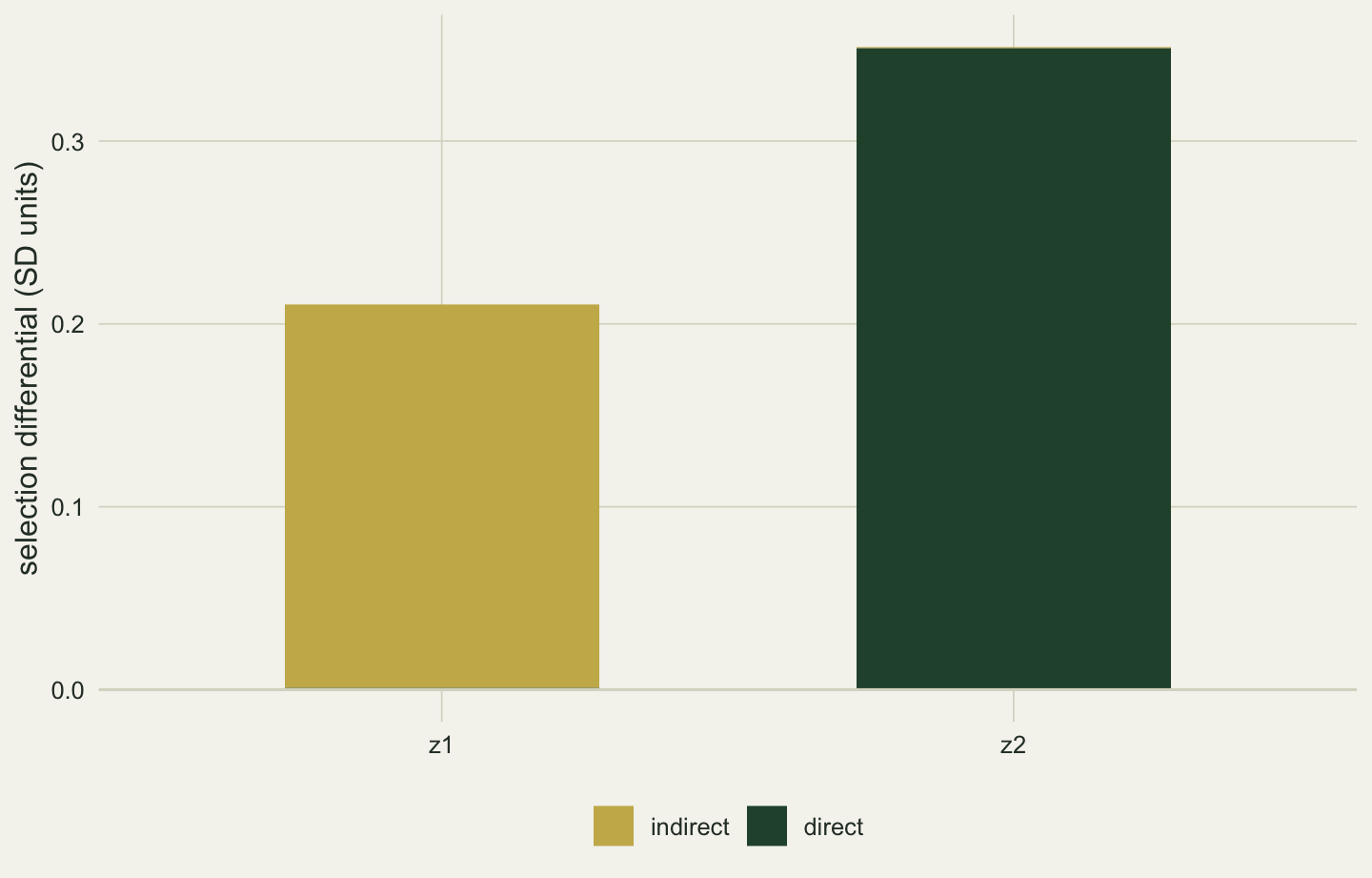
When the traits are uncorrelated P is diagonal, the indirect terms vanish, and each differential is its own gradient times its own variance; on standardised traits the two numbers then coincide. It follows that a study measuring one trait at a time is not measuring a smaller amount of selection. It is measuring a different quantity, the differential, whatever it calls it.
1.5 What the gradient estimates on a curved surface
The simulation above has a fitness surface that is not a plane. Expected offspring number rises exponentially with z2, so the change in fitness per unit of the trait is larger among large animals than among small ones. A linear regression fitted to it still returns a single slope, and it is fair to ask which slope that is.
For traits with a multivariate normal distribution the answer is exact. The least squares gradient equals the average, over the population, of the slope of the relative fitness surface,
\[ \boldsymbol\beta = \mathrm E \left[ \frac{\partial w}{\partial \mathbf z} \right], \]
a consequence of a property of the normal distribution known as Stein’s lemma (Stein 1981), and the reason Lande and Arnold could interpret beta as a gradient in the first place. On the exponential surface used here the slope of relative fitness at every point is 0.35 times the relative fitness at that point, so its average over the population is 0.35 exactly, whatever the spread of the trait. The regression recovers it. The condition is the normality of the trait, not of fitness, and it is easy to break.
set.seed(4311)
N_big <- 400000
z_norm <- rnorm(N_big)
w_norm <- exp(b2 * z_norm) / mean(exp(b2 * z_norm))
beta_norm <- unname(coef(lm(w_norm ~ z_norm))[2])

z_skew <- (rgamma(N_big, shape = 2) - 2) / sqrt(2)   # mean 0, variance 1, right-skewed
w_skew <- exp(b2 * z_skew) / mean(exp(b2 * z_skew))
beta_skew  <- unname(coef(lm(w_skew ~ z_skew))[2])
slope_skew <- mean(b2 * w_skew)
skew_z <- mean(z_skew^3)
With 400,000 individuals so that sampling error is out of the way, a normal trait on this surface gives a gradient of 0.350: the average slope. Give the trait the same mean and variance but a right skew, a skewness of 1.40, and the gradient comes back as 0.463, while the average slope of the surface is still 0.35. The regression is 32 per cent above the quantity it is usually read as. The long right tail of the trait sits on the steep part of the surface and pulls the least squares line up.
Nothing is wrong with the regression. beta is still the best linear description of how relative fitness varies with the trait in this sample, and it still predicts the change in mean correctly through S = P beta. What fails is the second reading, the one that treats beta as the local steepness of the fitness surface and carries it into models of evolution that assume that meaning. Where the skew comes from a trait that grows multiplicatively, as mass does, analysing it on the log scale before standardising removes most of it; the gradient is then a gradient on the log scale, and the paper has to say so. Where no transformation brings the trait near normality, the honest course is to report beta as the linear description it is and not to read it as a slope.
1.6 What the gradient cannot see
Two limits carry through the rest of Part I and are worth naming before the machinery gets any more elaborate.
The first is that the gradient separates direct from indirect selection only among the traits in the model. An unmeasured trait that affects fitness and correlates with a measured one leaves its selection on the measured trait, exactly as z2 left its selection on z1 in the differential. The gradient on the measured trait is then a mixture of its own selection and the selection on its missing partner, and the data contain no trace of the partner by which it could be detected. Chapter 3 measures how large the misattribution gets and what, short of measuring the partner, can be done about it.
The second is that everything in this chapter is phenotypic. A differential says which animals bred; it says nothing about whether their offspring will resemble them. That link needs the trait to be heritable and needs the covariance between the trait and fitness to run through the genes rather than through the environment, and Chapter 4 is where it enters. Before that, Chapter 2 takes the fitness surface seriously as a surface and asks about its curvature, which is the part of selection that holds a trait in place rather than moving it.
References
Lande R, Arnold SJ 1983. Evolution 37(6):1210-1226 (10.1111/j.1558-5646.1983.tb00236.x)
Hereford J, Hansen TF, Houle D 2004. Evolution 58(10):2133-2143 (10.1111/j.0014-3820.2004.tb01592.x)
Stein CM 1981. The Annals of Statistics 9(6):1135-1151 (10.1214/aos/1176345632)