amat <- function(sire, dam) {
  n <- length(sire)
  A <- matrix(0, n, n)
  for (i in seq_len(n)) {
    s <- sire[i]; d <- dam[i]
    if (i > 1L) {
      idx <- seq_len(i - 1L)
      v <- 0.5 * ((if (s > 0L) A[idx, s] else 0) + (if (d > 0L) A[idx, d] else 0))
      A[idx, i] <- v; A[i, idx] <- v
    }
    A[i, i] <- 1 + if (s > 0L && d > 0L) 0.5 * A[s, d] else 0
  }
  A
}
# restricted log-likelihood at absolute variances s = (V_A, V_N, V_R), intercept only
reml_ll <- function(y, Ao, Zn, s) {
  n <- length(y)
  V <- s[1] * Ao + s[3] * diag(n)
  if (!is.null(Zn)) V <- V + s[2] * Zn
  ch <- chol(V)
  Viy <- backsolve(ch, forwardsolve(t(ch), y))
  Vi1 <- backsolve(ch, forwardsolve(t(ch), rep(1, n)))
  s11 <- sum(Vi1)
  -0.5 * (2 * sum(log(diag(ch))) + log(s11) + sum(y * Viy) - sum(y * Vi1)^2 / s11)
}
# the same with V_R profiled out; r = (V_A / V_R, V_N / V_R)
reml_prof <- function(y, Ao, Zn, r) {
  n <- length(y)
  H <- diag(n) + r[1] * Ao
  if (!is.null(Zn)) H <- H + r[2] * Zn
  ch <- chol(H)
  Hiy <- backsolve(ch, forwardsolve(t(ch), y))
  Hi1 <- backsolve(ch, forwardsolve(t(ch), rep(1, n)))
  s11 <- sum(Hi1); nm <- n - 1
  ypy <- sum(y * Hiy) - sum(y * Hi1)^2 / s11
  list(ll = -0.5 * (nm * log(ypy / nm) + 2 * sum(log(diag(ch))) + log(s11) + nm),
       vr = ypy / nm)
}
fit_a <- function(y, Ao) {                   # animal model, no nest term
  o <- optimize(function(lr) -reml_prof(y, Ao, NULL, c(exp(lr), 0))$ll, c(-10, 4), tol = 1e-4)
  ra <- exp(o$minimum); p <- reml_prof(y, Ao, NULL, c(ra, 0))
  c(va = ra * p$vr, vn = 0, vr = p$vr, h2 = ra / (1 + ra), ll = p$ll)
}
fit_an <- function(y, Ao, Zn, start = c(-1.2, -1.2)) {   # with a nest term
  clamp <- function(lr) exp(pmax(pmin(lr, 4), -10))
  o <- optim(start, function(lr) -reml_prof(y, Ao, Zn, clamp(lr))$ll,
             method = "Nelder-Mead", control = list(reltol = 1e-6))
  r <- clamp(o$par); p <- reml_prof(y, Ao, Zn, r); tot <- (1 + sum(r)) * p$vr
  c(va = r[1] * p$vr, vn = r[2] * p$vr, vr = p$vr,
    h2 = r[1] * p$vr / tot, c2 = r[2] * p$vr / tot, ll = p$ll)
}
# the profiled and the absolute likelihood agree at the same variances
set.seed(909)
y_chk <- rnorm(10); A_chk <- amat(c(0, 0, rep(1, 10)), c(0, 0, rep(2, 10)))[3:12, 3:12]
Z_chk <- outer(rep(1:2, each = 5), rep(1:2, each = 5), "==") * 1
p_chk <- reml_prof(y_chk, A_chk, Z_chk, c(0.5, 0.3))
stopifnot(abs(p_chk$ll - reml_ll(y_chk, A_chk, Z_chk, p_chk$vr * c(0.5, 0.3, 1))) < 1e-9)9 Maternal effects and the shared nest
Chapter 8 ranked pedigrees by how precisely they pin down V_A, and the full-sib design came out well: families of close relatives, each family a handful of strong within-family contrasts, beat a design with many more related pairs. That ranking came with a condition written into the simulation. Every animal had an environment of its own, so the only reason two full sibs resembled each other was the half of their breeding values they shared. In a nest-box study that condition fails on the first day. Full sibs share a box, a pair of provisioning parents, a patch of wood and the weather of one fortnight, and every one of those makes them alike in the same way that shared genes do.
This chapter puts that shared environment into the simulation and measures what it does to an animal model that does not know about it. A nest effect left out arrives in V_A, doubled. Adding the missing term helps only if some relatives were reared apart, and with full sibs alone the data cannot choose between the two explanations at all. The parent-offspring regression of Chapter 4 escapes the nest and is inflated instead by what a mother passes to her young through her own phenotype, an effect that also travels down the pedigree where a nest term cannot follow.
9.1 Two sources of resemblance
The animal model of Chapter 7 has one random effect that makes relatives alike. The extended model adds a second, an effect of the nest in which each animal was reared:
\[ \mathbf y = \mu + \mathbf a + \mathbf Z \mathbf n + \mathbf e, \qquad \mathbf V = \mathbf A V_A + \mathbf Z \mathbf Z' V_N + \mathbf I V_R , \]
where Z assigns animals to nests, so that \(\mathbf Z \mathbf Z'\) is one for every pair reared in the same box and zero otherwise, and V_N is the variance among nests. Two full sibs from one box then covary by \(\tfrac12 V_A + V_N\), and a model without the nest term has only \(\tfrac12 V_A\) with which to reproduce that covariance.
The code rebuilds A with the recursion of Chapter 7 and writes the restricted likelihood of an intercept-only model twice: at absolute variances, and with V_R profiled out for fitting, which leaves the ratios \(V_A / V_R\) and \(V_N / V_R\) to the optimiser on the log scale. The two forms are checked against each other.
Two designs of the same size are compared. In the first every sire has one dam, so the only relatives are full sibs and every family is a nest. In the second every sire has several dams, which adds paternal half sibs, reared in different boxes.
make_design <- function(n_sire, dams_per_sire, k) {
  n_dam <- n_sire * dams_per_sire; n_off <- n_dam * k
  n_ped <- n_sire + n_dam + n_off
  sire <- integer(n_ped); dam <- integer(n_ped)
  off <- n_sire + n_dam + seq_len(n_off)
  sire[off] <- rep(rep(seq_len(n_sire), each = dams_per_sire), each = k)
  dam[off] <- rep(n_sire + seq_len(n_dam), each = k)
  A <- amat(sire, dam)
  list(L = t(chol(A)), Ao = A[off, off], off = off, n_ped = n_ped,
       nest = rep(seq_len(n_dam), each = k), n_off = n_off, n_nest = n_dam)
}
zz_of <- function(nest) outer(nest, nest, "==") * 1
sim_y <- function(d, va, vn, vr, nest = d$nest) {
  a <- as.vector(d$L %*% rnorm(d$n_ped)) * sqrt(va)
  a[d$off] + rnorm(max(nest), 0, sqrt(vn))[nest] + rnorm(d$n_off, 0, sqrt(vr))
}
k_off <- 4L; n_sire_fs <- 25L; n_sire_hs <- 5L; dps_hs <- 5L
fs <- make_design(n_sire_fs, 1L, k_off)     # every sire has one dam: full sibs only
hs <- make_design(n_sire_hs, dps_hs, k_off) # every sire has several dams: half sibs too
Z_fs <- zz_of(fs$nest); Z_hs <- zz_of(hs$nest)
V_A <- 0.3                                  # total variance held at 1 throughout
h2_true <- V_A
pairs_of <- function(Ao) table(round(Ao[upper.tri(Ao)], 4))
cls_fs <- pairs_of(fs$Ao); cls_hs <- pairs_of(hs$Ao)
stopifnot(fs$n_off == hs$n_off, cls_fs[["0.5"]] == cls_hs[["0.5"]], length(cls_fs) == 2L)
Both designs have 100 chicks in 25 nests of 4. The full-sib design contains 150 pairs at relatedness one half and nothing between that and zero. The half-sib design, 5 sires with 5 dams each, contains the same 150 full-sib pairs and 800 paternal half-sib pairs at a quarter. The additive variance is 0.30 and the nest variance is taken out of the residual, so the total stays at one and the true h^2 is 0.30 throughout the next two sections.
9.2 A nest term left out
The first experiment raises the true nest variance in steps and fits the animal model with and without the nest term to both designs.
set.seed(9091)
n_rep_grid <- 160L; vn_grid <- c(0, 0.1, 0.2, 0.3, 0.4)
grid_out <- NULL
for (vn in vn_grid) {
  vr <- 1 - V_A - vn
  m <- matrix(NA_real_, n_rep_grid, 5)
  for (i in seq_len(n_rep_grid)) {
    y_f <- sim_y(fs, V_A, vn, vr); y_h <- sim_y(hs, V_A, vn, vr)
    m[i, 1] <- fit_a(y_f, fs$Ao)["h2"]
    m[i, 2] <- fit_a(y_h, hs$Ao)["h2"]
    m[i, 3:5] <- fit_an(y_h, hs$Ao, Z_hs)[c("h2", "c2", "vn")]
  }
  if (vn == 0) cell0 <- m
  grid_out <- rbind(grid_out, data.frame(vn = vn, fs_no = mean(m[, 1]), hs_no = mean(m[, 2]),
    hs_with = mean(m[, 3]), hs_c2 = mean(m[, 4]),
    se_fs_no = sd(m[, 1]) / sqrt(n_rep_grid), se_hs_with = sd(m[, 3]) / sqrt(n_rep_grid)))
}
slope_fs <- unname(coef(lm(fs_no ~ vn, grid_out[1:4, ]))[2])
slope_hs <- unname(coef(lm(hs_no ~ vn, grid_out[1:4, ]))[2])
# with unrelated families the full-sib covariance V_A / 2 + V_N must be matched by V_A' / 2
va_implied <- V_A + 2 * vn_grid
stopifnot(all(abs((va_implied / 2) - (V_A / 2 + vn_grid)) < 1e-12))
prem <- c(mean_no = mean(cell0[, 2]), mean_with = mean(cell0[, 3]),
          sd_no = sd(cell0[, 2]), sd_with = sd(cell0[, 3]),
          rmse_no = sqrt(mean((cell0[, 2] - h2_true)^2)),
          rmse_with = sqrt(mean((cell0[, 3] - h2_true)^2)),
          at0 = mean(cell0[, 5] < 1e-3))
Each step holds 160 replicates of each design. With no nest effect the model without a nest term is right, as it should be: its mean estimate on the full-sib design is 0.301 against a true 0.30. At a nest variance of 0.20 it returns 0.686, and at 0.30 it returns 0.837, calling most of the variation in a trait with a heritability of 0.30 genetic. A straight line through the first four steps rises by 1.80 units of heritability per unit of nest variance. The expected rate is two, and the reason is arithmetic. With unrelated families, the only resemblance in the data is between full sibs, and it amounts to \(\tfrac12 V_A + V_N\). A model that has only the additive term must reproduce that with half of its own V_A, so the additive variance it settles on is \(V_A + 2V_N\). The shared environment is not merely credited to the genes; it is divided by the relatedness of the pairs that display it, which doubles it. The measured rate falls short of two partly because a heritability cannot exceed one, and the implied value is already 0.90 at the fourth step and 1.10 at the last.
The obvious hope is that paternal half sibs would protect the estimate, since they offer a view of V_A from pairs that never shared a box. They do not. The half-sib design without a nest term returns 0.726 at a nest variance of 0.20, and its slope over the same steps is 2.03, no smaller than the full-sib slope. A model with a single source of resemblance allows the broods of one sire to differ by a quarter of V_A and no more, so the nest variance that separates those broods can only be read as extra V_A, and seen from that contrast it is multiplied by four rather than two. Adding half sibs to a model without the nest term leaves the inflation no smaller, and here slightly larger. Half sibs make the correct model estimable; they do nothing for the incorrect one.
lab_mod <- c("full sibs, no nest term", "half sibs, no nest term", "half sibs, nest term")
fa <- data.frame(vn = rep(grid_out$vn, 3),
                 h2 = c(grid_out$fs_no, grid_out$hs_no, grid_out$hs_with),
                 model = factor(rep(lab_mod, each = nrow(grid_out)), levels = lab_mod))
ggplot(fa, aes(vn, h2, colour = model, shape = model)) +
  geom_hline(yintercept = h2_true, linetype = "dashed", colour = te_sage) +
  geom_line(linewidth = 0.8) + geom_point(size = 2.6) +
  scale_colour_manual(values = c(te_rust, te_gold, te_forest), name = NULL) +
  scale_shape_manual(values = c(16, 17, 15), name = NULL) +
  scale_y_continuous(limits = c(0, 1)) +
  labs(x = "true nest variance", y = "mean estimated heritability") +
  theme_book()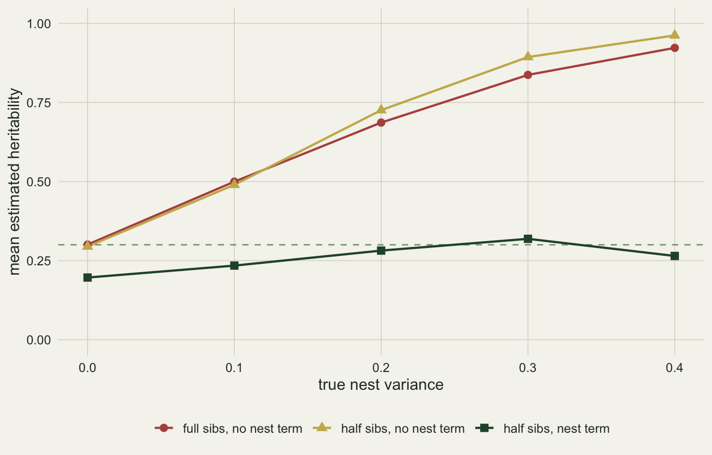
The model with the nest term, fitted to the half-sib design, is the low line in the figure above. Its mean estimate stays between 0.196 and 0.319 across the whole range, while its estimated nest share of the variance follows the truth from 0.050 to 0.398. It is pointed at the right place without being accurate. With 100 chicks it sits below the truth at 4 of the 5 steps, and at the first step the shortfall of 0.104 is 7 times its Monte Carlo standard error, far too large to be noise.
That first step, where the true nest variance is zero, also prices the term when it is not needed. Without it the half-sib estimate averages 0.295; with it, 0.196. In 55 per cent of replicates the nest variance sits at its boundary of zero. In the rest, sampling noise has made some broods more alike than their genes explain, and the nest term takes that excess from V_A; when broods are less alike than expected, it has nothing to give back. The root mean squared error hardly moves, 0.212 against 0.216, so the premium is paid in the value that ends up in the table. A term for something relatives share takes additive variance with it whenever the two can trade, the problem Chapter 6 raised for a territory that relatives hold in common.
9.3 What full sibs cannot say
Fitting the nest term to the full-sib design as well does not work, and the reason is not power. In that design the covariance matrix has only two distinct entries within a brood: the variance of a chick, \(V_A + V_N + V_R\), and the covariance of two sibs, \(\tfrac12 V_A + V_N\). Between broods it is zero. Two numbers cannot determine three variances, and any two triples that agree on both give the same likelihood exactly.
set.seed(9092)
demo_v <- c(V_A, 0.2, 0.5)
y_fs1 <- sim_y(fs, demo_v[1], demo_v[2], demo_v[3])
y_hs1 <- sim_y(hs, demo_v[1], demo_v[2], demo_v[3])
# two triples with the same sib covariance and the same total variance
t1 <- c(0.2, 0.15, 0.6); t2 <- c(0.5, 0, 0.45)
stopifnot(abs((t1[1] / 2 + t1[2]) - (t2[1] / 2 + t2[2])) < 1e-12,
          abs(sum(t1) - sum(t2)) < 1e-12)
ll_t <- c(reml_ll(y_fs1, fs$Ao, Z_fs, t1), reml_ll(y_fs1, fs$Ao, Z_fs, t2))
stopifnot(abs(diff(ll_t)) < 1e-9)
ll_t_hs <- c(reml_ll(y_hs1, hs$Ao, Z_hs, t1), reml_ll(y_hs1, hs$Ao, Z_hs, t2))

n_start <- 60L
st <- cbind(runif(n_start, -4, 1), runif(n_start, -4, 1))
multi <- function(y, Ao, Zn) t(apply(st, 1, function(s) fit_an(y, Ao, Zn, s)))
Q_fs <- multi(y_fs1, fs$Ao, Z_fs); Q_hs <- multi(y_hs1, hs$Ao, Z_hs)
ridge_slope <- unname(coef(lm(Q_fs[, "vn"] ~ Q_fs[, "va"]))[2])
ll_rng <- c(fs = diff(range(Q_fs[, "ll"])), hs = diff(range(Q_hs[, "ll"])))
On one simulated full-sib data set, a triple with an additive variance of 0.20 and a nest variance of 0.15, and another with 0.50 and none, have restricted log-likelihoods equal to the precision of the arithmetic, which the code checks. One says the box does much of the work, the other that it does nothing. On a half-sib data set drawn from the same variances the same two triples differ by 1.53 log-likelihood units.
An optimiser meets this as a ridge. Started from 60 scattered values on the one full-sib data set, the fit returns additive variances from 0.025 to 0.570 and heritabilities from 0.023 to 0.536, with log-likelihoods that differ by no more than 0.0003 units, the tolerance of the optimiser. Every one of them is a maximum. They lie on a line of slope -0.499 in the plane of the two variances, the arithmetic of the sib covariance made visible: each unit of additive variance added is paid for by half a unit of nest variance removed.
fc <- rbind(data.frame(va = Q_fs[, "va"], vn = Q_fs[, "vn"], design = "full sibs only"),
            data.frame(va = Q_hs[, "va"], vn = Q_hs[, "vn"], design = "with paternal half sibs"))
ggplot(fc, aes(va, vn)) +
  geom_point(colour = te_forest, size = 2, alpha = 0.7) +
  annotate("point", x = demo_v[1], y = demo_v[2], colour = te_rust, shape = 4, size = 3.4, stroke = 1.3) +
  facet_wrap(~ design) +
  labs(x = "estimated additive variance", y = "estimated nest variance") +
  theme_book()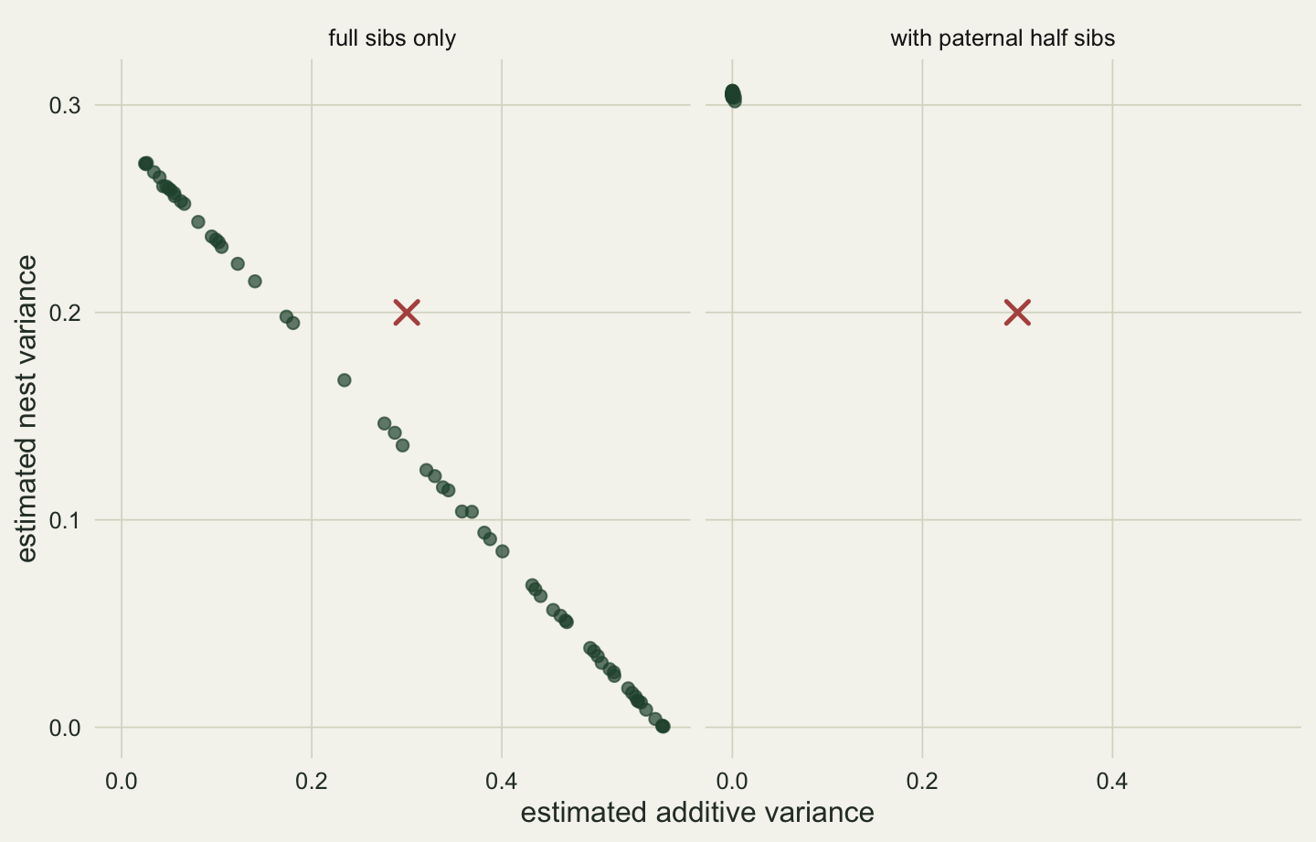
On the half-sib data set all 60 runs agree, their log-likelihoods within 0.006 units, on an additive variance of at most 0.003. That is not a flattering answer for a trait simulated at 0.30; it is the sampling spread of Chapter 7 on a small design. The model is identified and the estimate is poor. On the full-sib data no estimate exists to be poor.
A routine analysis does not run sixty starts. It fits each data set once, from a default starting value, and a replicate study of that habit looks like good news.
set.seed(9093)
n_rep_fix <- 150L
fix_h2 <- hs_h2 <- dll <- numeric(n_rep_fix)
for (i in seq_len(n_rep_fix)) {
  y_f <- sim_y(fs, demo_v[1], demo_v[2], demo_v[3])
  y_h <- sim_y(hs, demo_v[1], demo_v[2], demo_v[3])
  a0 <- fit_an(y_f, fs$Ao, Z_fs)                 # the default start, every time
  fix_h2[i] <- a0["h2"]; dll[i] <- a0["ll"] - fit_a(y_f, fs$Ao)["ll"]
  hs_h2[i] <- fit_an(y_h, hs$Ao, Z_hs, runif(2, -3, 0))["h2"]
}
h2_start <- exp(-1.2) / (1 + 2 * exp(-1.2))    # heritability implied by the default start
alpha <- 0.05
lrt_crit <- qchisq(1 - 2 * alpha, 1)            # boundary mixture threshold
n_sig <- sum(2 * dll > lrt_crit)

set.seed(9094)
n_rep_big <- 100L; big_v <- c(V_A, 0.45, 0.25)
dll_big <- replicate(n_rep_big, {
  y_f <- sim_y(fs, big_v[1], big_v[2], big_v[3])
  fit_an(y_f, fs$Ao, Z_fs)["ll"] - fit_a(y_f, fs$Ao)["ll"]
})
r_fs_big <- big_v[1] / 2 + big_v[2]
sig_big <- mean(2 * dll_big > lrt_crit)
Across 150 full-sib data sets simulated with a nest variance of 0.20, the heritability from the default start has a standard deviation of 0.032. The half-sib design, the same size and correctly specified, gives 0.286, 8.9 times larger. Read as precision, the full-sib design wins easily, yet it is the one design that cannot estimate the heritability. The full-sib estimate averages 0.198, close to the 0.188 implied by the starting value: on a ridge the optimiser stops wherever its first steps leave it. This is the unrelated design of Chapter 8 again, where a flat likelihood produced a spread of zero that meant no information at all.
The likelihood-ratio test is no help either. Against the boundary threshold of 2.71 from Chapter 6, the nest term was significant in 0 of the 150 full-sib data sets, although the nest variance was two thirds of the additive variance; its largest gain in log-likelihood was 0.991 units and its mean gain 0.020. The test is blind, not weak: the model without the nest term is a point on the ridge and reaches the same maximum, unless the sib covariance exceeds half the phenotypic variance, which additive inheritance alone cannot produce. With a nest variance of 0.45 the sib correlation is 0.60, and the test now rejects the smaller model in 28 per cent of 100 replicates. A shared environment strong enough to break that ceiling is sometimes visible in full-sib data. Anything weaker is not.
9.4 The parent-offspring regression
Chapter 4 estimated h^2 as the slope of offspring on midparent, with a warning that shared environments inflate it. The nest of the previous sections does not: it is shared by siblings, not by a chick and its parents, who grew up in boxes of their own. The environment that enters the regression is one that links the generations, and a common one in birds and mammals is a mother whose own phenotype shapes her young, as when a large female lays larger eggs. The simulation below lets each chick’s phenotype include m times its mother’s phenotype and regresses chicks on their parents.
set.seed(9095)
n_fam <- 5000; V_N_po <- 0.2; V_R_po <- 1 - V_A - V_N_po
parent <- function(n) { a <- rnorm(n, 0, sqrt(V_A)); list(a = a, z = a + rnorm(n, 0, sqrt(1 - V_A))) }
sires <- parent(n_fam); dams <- parent(n_fam)
mid <- (sires$z + dams$z) / 2
a_off <- function() (sires$a + dams$a) / 2 + rnorm(n_fam, 0, sqrt(V_A / 2))
nest <- rnorm(n_fam, 0, sqrt(V_N_po))
# two chicks per nest, nest effect only
o1 <- a_off() + nest + rnorm(n_fam, 0, sqrt(V_R_po))
o2 <- a_off() + nest + rnorm(n_fam, 0, sqrt(V_R_po))
po_nest <- coef(summary(lm(o1 ~ mid)))[2, 1:2]
sib_nest <- 2 * cor(o1, o2)
# a maternal effect through the mother's phenotype, with and without fostering
m_pos <- 0.4; m_neg <- -0.25
foster <- sample(n_fam)                            # each brood raised by a random mother
po_mat <- function(m, host) {
  o <- a_off() + m * dams$z[host] + rnorm(n_fam, 0, sqrt(1 - V_A))
  c(mid = unname(coef(lm(o ~ mid))[2]), dam = unname(coef(lm(o ~ dams$z))[2]),
    sire = unname(coef(lm(o ~ sires$z))[2]), host = unname(coef(lm(o ~ dams$z[host]))[2]))
}
po_pos <- po_mat(m_pos, seq_len(n_fam)); po_neg <- po_mat(m_neg, seq_len(n_fam))
po_fost <- po_mat(m_pos, foster)
# expected midparent slope when the mother's phenotype enters her young's: h2 + m
po_se <- po_nest[[2]]
stopifnot(abs(po_pos[["mid"]] - (h2_true + m_pos)) < 5 * po_se,
          abs(po_neg[["mid"]] - (h2_true + m_neg)) < 5 * po_se,
          abs(po_fost[["mid"]] - h2_true) < 5 * po_se,
          abs(po_fost[["host"]] - m_pos) < 5 * po_se)
With 5,000 families and a nest variance of 0.20 shared by two chicks per brood, the midparent slope is 0.277 (standard error 0.020) against a true 0.30. The same chicks, read as full sibs, give twice their intraclass correlation as 0.683. The nest inflates the sib estimate and leaves the parent-offspring estimate alone.
The maternal effect reverses that. With m = 0.40 the midparent slope is 0.698. The algebra is short: the mother’s phenotype now enters the chick directly, which adds \(m V_P\) to the covariance of chick and mother, and the midparent slope becomes \(h^2 + m\), which the chunk checks against the simulation. The whole maternal coefficient is added to the heritability, and the estimate here is more than twice the truth. A compensating effect, m = -0.25, pushes the slope down to 0.041, close to zero for a trait whose true heritability is 0.30.
The classical diagnostic separates the two parents. Regressed on the sire alone, the chicks give 0.133, close to the \(\tfrac12 h^2\) = 0.150 expected from genes; regressed on the dam alone, 0.558. A dam slope well above the sire slope is the signature of a maternal effect (Falconer and Mackay 1996). Cross-fostering removes the effect from the regression. When every brood is raised by a mother drawn at random, the slope on the genetic midparent is 0.291, back at the heritability, and the slope on the foster mother is 0.411, an estimate of m itself. The design that answers the question is the one that breaks the link between the mother who supplies the genes and the mother who supplies the care.
9.5 Moving chicks between nests
The same move repairs the animal model. Swapping chicks between boxes after hatching stops the nest being a synonym for the family, and the model can then assign resemblance to whichever grouping carries it. The simulation fosters a fraction of the chicks in the full-sib design, the one that could not identify the nest term.
move <- function(nest, f) {
  n <- length(nest); k <- round(f * n)
  if (k < 2) return(nest)
  idx <- sample.int(n, k); nest[idx] <- nest[sample(idx)]; nest
}
set.seed(9096)
f_grid <- c(0, 0.1, 0.25, 0.5, 0.75, 1); n_rep_f <- 150L
fost_out <- NULL
for (f in f_grid) {
  m <- matrix(NA_real_, n_rep_f, 2)
  for (i in seq_len(n_rep_f)) {
    nn <- move(fs$nest, f)
    y_f <- sim_y(fs, demo_v[1], demo_v[2], demo_v[3], nest = nn)
    m[i, ] <- fit_an(y_f, fs$Ao, zz_of(nn))[c("h2", "c2")]
  }
  fost_out <- rbind(fost_out, data.frame(f = f, mean_h2 = mean(m[, 1]), sd_h2 = sd(m[, 1]),
                                         sd_c2 = sd(m[, 2])))
}
mc_sd <- fost_out$sd_h2 / sqrt(2 * (n_rep_f - 1))   # Monte Carlo error of a standard deviation
fd <- rbind(data.frame(f = fost_out$f, s = fost_out$sd_h2, what = "heritability"),
data.frame(f = fost_out$f, s = fost_out$sd_c2, what = "nest share"))
ggplot(fd, aes(f, s, colour = what, shape = what)) +
geom_line(data = fd[fd$f > 0, ], linewidth = 0.8) + geom_point(size = 2.6) +
scale_colour_manual(values = c(te_forest, te_gold), name = NULL) +
scale_shape_manual(values = c(16, 17), name = NULL) +
expand_limits(y = 0) +
labs(x = "fraction of chicks fostered", y = "standard deviation across replicates") +
theme_book()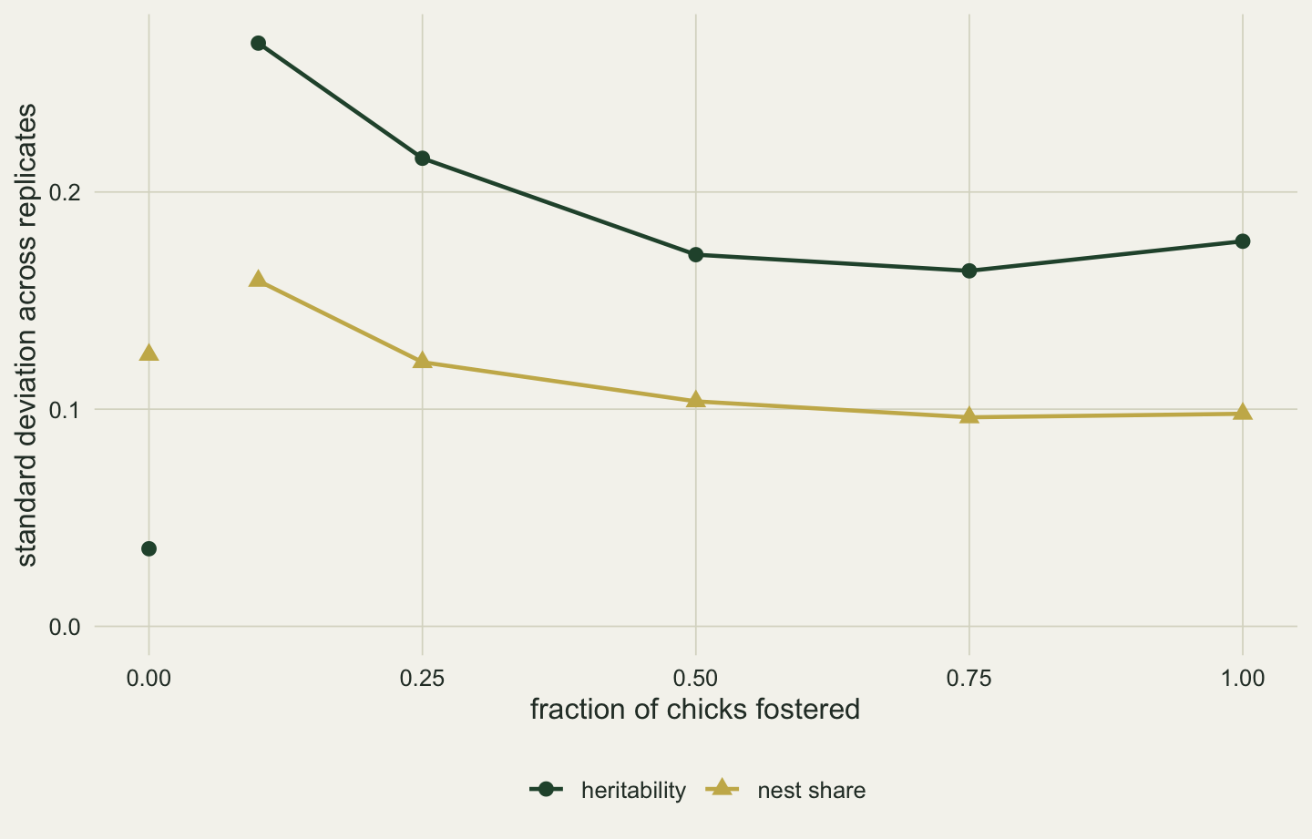
Fostering a tenth of the chicks is enough to make the model estimable: across 150 replicates the mean heritability is 0.295, against 0.30, although its standard deviation of 0.269 shows how little a tenth buys in precision. A quarter fostered brings the spread to 0.216 and a half to 0.171. Beyond that the curve is flat: 0.164 at three quarters and 0.177 with every chick’s nest reassigned, differences of the same size as their Monte Carlo errors, about 0.010 each. Once half the brood has been moved, further moves add nothing that 150 replicates can detect.
The point at zero is the trap of the previous section: with nothing fostered the standard deviation is 0.036, the smallest in the experiment, and the mean is 0.199, sitting on the starting value again. A spread across replicates measures precision only for a parameter the design identifies.
9.6 A mother is not a nest
The nest effect simulated so far was drawn once per box, independently of everything else, exactly as the nest term assumes. The maternal effect of the last section is not. If a chick’s phenotype contains m times its mother’s, it contains m times her breeding value, and mothers are relatives too. The effect then passes down the pedigree instead of stopping at the nest. To see it, the next pedigree adds a generation of grandsires, so that the dams fall into groups of paternal half sisters, and mates each sire to one dam from each group.
n_gs <- 5L; dpg <- 5L; n_ms <- 5L
n_md <- n_gs * dpg; n_mo <- n_md * k_off
gsire <- seq_len(n_gs); msire <- n_gs + seq_len(n_ms)
mdam <- n_gs + n_ms + seq_len(n_md)
moff <- n_gs + n_ms + n_md + seq_len(n_mo)
n_mp <- max(moff)
sire_m <- dam_m <- integer(n_mp)
sire_m[mdam] <- rep(gsire, each = dpg)                       # dams are paternal half sisters
dam_of <- rep(as.vector(sapply(seq_len(n_ms), function(s)
  mdam[(seq_len(n_gs) - 1L) * dpg + s])), each = k_off)      # each sire mates one dam per group
sire_m[moff] <- rep(msire, each = n_gs * k_off); dam_m[moff] <- dam_of
Am <- amat(sire_m, dam_m); Lm <- t(chol(Am)); Amo <- Am[moff, moff]
Z_m <- zz_of(match(dam_of, mdam))
V_R_m <- 1 - V_A
same_dam <- outer(dam_of, dam_of, "==") * 1
# Willham's decomposition: direct, direct-maternal covariance, maternal genetic,
# maternal environment, residual
cov_willham <- function(m) V_A * Amo + m * V_A * (Am[moff, dam_of] + t(Am[moff, dam_of])) +
  m^2 * V_A * Am[dam_of, dam_of] + m^2 * V_R_m * same_dam + V_R_m * diag(n_mo)
# the same covariance from the linear map y = (offspring + m * dam) a + m e_dam + e
Po <- matrix(0, n_mo, n_mp); Po[cbind(seq_len(n_mo), moff)] <- 1
Pd <- matrix(0, n_mo, n_mp); Pd[cbind(seq_len(n_mo), dam_of)] <- 1
cov_map <- function(m) (Po + m * Pd) %*% Am %*% t(Po + m * Pd) * V_A +
  m^2 * V_R_m * same_dam + V_R_m * diag(n_mo)
stopifnot(max(abs(cov_willham(m_pos) - cov_map(m_pos))) < 1e-12,
          max(abs(cov_willham(m_neg) - cov_map(m_neg))) < 1e-12)
sim_mat <- function(m) {
  a <- as.vector(Lm %*% rnorm(n_mp)) * sqrt(V_A)
  zd <- a + rnorm(n_mp, 0, sqrt(V_R_m))                      # only the dams' entries are used
  a[moff] + m * zd[dam_of] + rnorm(n_mo, 0, sqrt(V_R_m))
}
cls <- round(Amo, 4); ut <- upper.tri(cls); lv <- sort(unique(cls[ut]))
msk <- lapply(lv, function(l) which(ut & cls == l))
set.seed(9097)
n_rep_cov <- 500L; n_rep_mfit <- 120L
mat_out <- NULL; cov_out <- NULL
for (m in c(m_pos, m_neg)) {
  cv <- t(replicate(n_rep_cov, { y <- sim_mat(m); cp <- outer(y, y)
    sapply(msk, function(w) mean(cp[w])) }))
  cw <- cov_willham(m)
  cov_out <- rbind(cov_out, data.frame(m = m, r = lv, genes = lv * V_A,
    predicted = sapply(msk, function(w) mean(cw[w])), observed = colMeans(cv)))
  res <- t(replicate(n_rep_mfit, { y <- sim_mat(m)
    c(fit_an(y, Amo, Z_m)[c("va", "vn", "h2")], no = fit_a(y, Amo)[["h2"]]) }))
  vp <- mean(diag(cw))
  mat_out <- rbind(mat_out, data.frame(m = m, vp = vp, h2 = V_A / vp,
    va_hat = mean(res[, 1]), h2_with = mean(res[, 3]), h2_no = mean(res[, 4]),
    at_zero = mean(res[, 2] < 1e-3)))
}
cp <- cov_out[cov_out$m == m_pos, ]; cn <- cov_out[cov_out$m == m_neg, ]
stopifnot(identical(lv, c(0, 0.0625, 0.25, 0.5)))
The 100 chicks now fall into three classes of relative besides the unrelated: full sibs at one half, paternal half sibs at a quarter whose mothers are unrelated, and pairs at 0.0625 whose mothers are half sisters. Willham (1972) wrote the covariance between relatives under a maternal effect as a direct additive part, a maternal genetic part scaled by the relatedness of the two mothers, a covariance between one animal’s direct and the other’s mother’s maternal breeding value, and a maternal environment shared by one mother’s young. The effect simulated here is the special case with maternal genetic variance \(m^2 V_A\), direct-maternal covariance \(m V_A\) and maternal environment \(m^2 V_R\); the chunk builds the covariance that way and again from the simulation’s linear map, and the two agree to the precision of the arithmetic.
The class covariances show where the effect goes. With m = 0.40, full sibs are predicted to covary by 0.430 against 0.150 from genes alone, and over 500 simulated data sets they do, at 0.427. A nest term can absorb that. The chicks of half-sister mothers are predicted to covary by 0.061 where genes predict 0.019, and they are observed at 0.066: 3.5 times the genetic value, in different boxes under different mothers. Only the paternal half sibs, at 0.075 against 0.075, are untouched, because their mothers are unrelated.
mp <- mat_out[mat_out$m == m_pos, ]; mn <- mat_out[mat_out$m == m_neg, ]So the model with a nest term is pulled two ways. With m = 0.40 the true heritability, V_A over a phenotypic variance that the maternal path has raised to 1.28, is 0.234. The model with the nest term returns 0.298 and an additive variance of 0.412 against 0.30: the nest term took the within-brood excess, and the excess between the broods of related mothers had nowhere to go but V_A. Without the nest term the estimate is 0.682. With the compensating m = -0.25, full sibs are less alike than their genes alone would make them, 0.133 against 0.150. A variance cannot be negative, so the nest term sits at zero in 52 per cent of fits, and the model absorbs the shortfall by shrinking V_A to 0.202, a heritability of 0.204 against a true 0.304. Here the model without the nest term does better, at 0.291.
A nest effect can only inflate a heritability that omits it; a maternal effect can move it either way, and a nest term does not reveal the sign. What does is the regression on each parent separately, which needs mothers measured for the same trait, or a maternal genetic effect in Willham’s form: a second breeding value for every mother, with its own variance and a covariance with the direct one, fitted on a pedigree that links mothers across generations and ideally on fostered young. This chapter does not fit that model. It adds a maternal genetic variance and a direct-maternal covariance to the three variances fitted here, and on 100 chicks those three were already hard to pin down.
9.7 What the pedigree has to contain
Every finding here is about design rather than software. An omitted nest enters V_A nearly doubled, half sibs make the nest term estimable without protecting a model that leaves it out, fostering makes it estimable in the one design that could not identify it, and with full sibs alone the starting value chooses the answer. The parent-offspring regression escapes the nest and is caught by the mother’s phenotype, which dam and sire slopes or a fostering design expose, and a maternal effect carried by the mother’s breeding value reaches relatives that a nest term never sees. Two habits follow: refit variance components from scattered starts and compare likelihoods rather than estimates, and treat an unusually stable estimate as a question about identification. Kruuk (2004) describes the long-term studies in which these terms are fitted, and Lynch and Walsh (1998) give the full algebra of maternal-effect models.
All of this assumes that the analysis stops at the variance components, and most do not. The predicted breeding values of Chapter 7 are taken out and regressed on year or on fitness, and Chapter 4, while naming the covariance of fitness with breeding values as the remedy for the stasis paradox, warned against exactly that second step. A breeding value predicted by a model that has absorbed a nest effect or a maternal effect carries that environment with it, and even a correctly specified model hands on predictions that are shrunk, correlated and unequally reliable. Chapter 10 measures what those second analyses report, and what the animal model has to be asked directly instead.
References
Willham RL 1972. Journal of Animal Science 35(6):1288-1293 (10.2527/jas1972.3561288x)
Falconer DS, Mackay TFC 1996. Introduction to Quantitative Genetics, 4th ed. Longman. ISBN 978-0582243026
Kruuk LEB 2004. Philosophical Transactions of the Royal Society B 359(1446):873-890 (10.1098/rstb.2003.1437)
Lynch M, Walsh B 1998. Genetics and Analysis of Quantitative Traits. Sinauer. ISBN 978-0878934812