5  The G matrix and correlated response

Beak depth and beak width in a finch, flowering date and height in a plant, body mass and wing length in almost anything: traits measured on the same organism share genes, and a gene that raises one of them often raises another. Selection on one trait therefore moves the others, and whether a population can reach the combination of traits that selection favours depends less on how much genetic variation each trait has than on how that variation is arranged across traits.

The arrangement is a matrix. This chapter replaces the heritability of Chapter 4 with the additive genetic covariance matrix G, reads the matrix through its eigenvectors, and measures two consequences: a response that points somewhere other than where selection pushed, and a response that barely happens at all even though every trait is heritable. It ends on a practical problem that shapes Part III. The directions in which G holds little variance are the ones that matter most for constraint, and they are the ones a study of realistic size estimates worst.

5.1 The multivariate breeder’s equation

With several traits the additive variances and the covariances between breeding values form a matrix G, the phenotypic variances and covariances form P, and selection is described by the vector of gradients beta from Chapter 1. Lande (1979) showed that the change in the vector of trait means across one generation is

\[ \Delta \bar{\mathbf z} = \mathbf G \boldsymbol\beta = \mathbf G \mathbf P^{-1} \mathbf S . \]

The single-trait breeder’s equation is the one-dimensional case, where G P^-1 is V_A / V_P, the heritability. The multivariate form separates the two things that determine a response more cleanly than the scalar form can. Selection is in beta, measured on the phenotypes. Inheritance is in G, a property of the population. The response is their product, and a matrix times a vector can point anywhere.

5.2 Reading G through its eigenvectors

Take two traits with equal additive variances and a strong positive genetic correlation.

r_g <- 0.7
G <- matrix(c(1, r_g, r_g, 1), 2)
eg <- eigen(G)
g_max <- eg$vectors[, 1] * sign(eg$vectors[1, 1])
angle <- function(u, v) acos(sum(u * v) / sqrt(sum(u^2) * sum(v^2))) * 180 / pi

The genetic correlation is 0.70, and each trait on its own has as much additive variance as the other. The eigenvalues of G are 1.70 and 0.30. The leading eigenvector, usually called g_max, runs along the diagonal in which both traits increase together, and it holds 85 per cent of the additive variance. The perpendicular direction, one trait up and the other down, holds the rest. Schluter (1996) called g_max the genetic line of least resistance, on the argument that a population responds most readily along it and is deflected towards it when selected in any other direction. G is a covariance matrix, and its eigenvectors are exactly the principal components of the breeding values.

5.3 A correlated response

Select on the first trait alone and leave the second trait alone.

beta_A <- c(0.3, 0)
dz_A <- drop(G %*% beta_A)
defl_A <- angle(dz_A, beta_A)
off_gmax_A <- angle(dz_A, g_max)

With a gradient of 0.30 on the first trait, the response is 0.300 in that trait and 0.210 in the second, which experienced no direct selection. That second number is the correlated response. It points 35 degrees away from the direction of selection and only 10 degrees away from g_max: selection chose the target, and the genetic covariance steered the population towards the diagonal on the way.

A correlated response is not always welcome. If the second trait were under stabilising selection of its own, the correlated response would push it off its optimum, and selection on it would then pull back against the response in the first trait. Much of the evolutionary interest in G lies in this kind of tug between traits that share genes.

5.4 Constraint without a shortage of variation

Now let selection favour the first trait and disfavour the second by the same amount. That direction runs across the diagonal, the direction G holds least of.

beta_B <- c(0.3, -0.3)
dz_B <- drop(G %*% beta_B)
dz_B_indep <- drop(diag(diag(G)) %*% beta_B)
shrink <- 1 - sqrt(sum(dz_B^2)) / sqrt(sum(dz_B_indep^2))
evolv <- function(b, G) drop(t(b) %*% G %*% b) / sum(b^2)
e_A <- evolv(beta_A, G); e_B <- evolv(beta_B, G)

With gradients of 0.30 and -0.30, and the same additive variances but no genetic correlation, this selection would move the population by 0.424 in trait space. With the correlation it moves by 0.127, 70 per cent less. Each trait is as heritable as before, and each would respond readily to selection on its own. The combination selection is trying to build is the one the genes shared between the two traits make expensive.

Hansen and Houle (2008) put a number on this with the evolvability in the direction of selection, the additive variance along the unit vector of beta, beta' G beta / beta' beta. It is the quantity that sets the rate of response in a given direction. For selection on the first trait alone it is 1.000; for the antagonistic selection it is 0.300, the smaller eigenvalue exactly, because that selection points straight along the minor axis. As the direction of selection turns through a full circle, evolvability swings between the two eigenvalues, and the heritability of each trait, which is all a table of single-trait analyses would report, says nothing about where in that range a particular selection regime falls.

th <- seq(0, 180, length.out = 361)
ev <- vapply(th, function(a) evolv(c(cos(a * pi / 180), sin(a * pi / 180)), G), 0)
marks <- data.frame(th = c(0, 135), ev = c(e_A, e_B),
                    lab = c("trait 1 only", "antagonistic"))
ggplot(data.frame(th, ev), aes(th, ev)) +
  geom_hline(yintercept = G[1, 1], colour = te_sage, linetype = "dotted") +
  geom_line(colour = te_forest, linewidth = 0.9) +
  geom_point(data = marks, colour = te_rust, size = 2.6) +
  geom_text(data = marks, aes(label = lab), colour = te_body, size = 3.4,
            nudge_x = c(4, 0), nudge_y = c(-0.06, 0.08), hjust = c(0, 0.5)) +
  scale_x_continuous(breaks = seq(0, 180, 45)) +
  labs(x = "direction of selection (degrees from trait 1)",
       y = "evolvability along beta") +
  theme_book()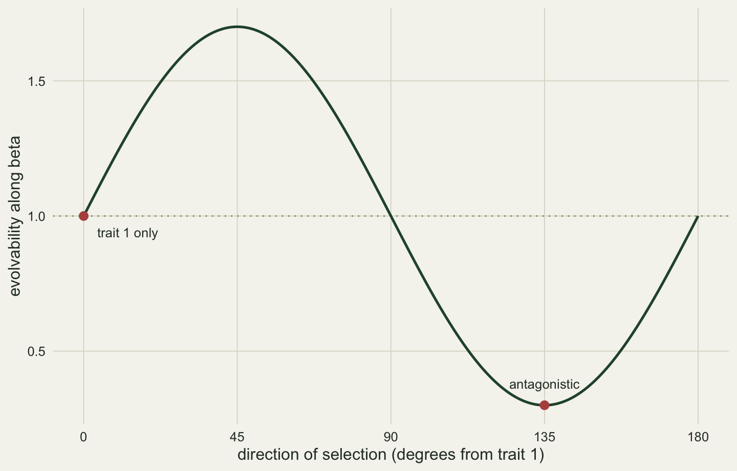

Figure 5.1: Additive genetic variance along the direction of selection (evolvability) as the direction turns through half a circle. The dotted line is the variance of each trait on its own. Selection on one trait alone and antagonistic selection are marked.

Walsh and Blows (2009) argued from exactly this geometry that multivariate adaptation is more often limited by directions of near-zero genetic variance than by any shortage of variance in individual traits. With two traits the argument is a curiosity. With ten or twenty traits, which is the realistic dimension of a phenotype, the smallest eigenvalues of G are routinely close to zero, and much of trait space is effectively out of reach.

5.5 The equation checked on individuals

The matrix equation is exact given G and beta. To see that it is also exact on a population of individuals, and to connect it back to Robertson’s form in Chapter 4, draw breeding values from G, add environmental deviations with their own correlation, and impose a fitness function on the phenotypes.

set.seed(433)
n <- 20000
E <- matrix(c(1, 0.2, 0.2, 1), 2)
a <- matrix(rnorm(2 * n), n) %*% chol(G)
z <- a + matrix(rnorm(2 * n), n) %*% chol(E)
P <- cov(z)
w <- pmax(1 + drop(z %*% beta_A), 0); w <- w / mean(w)
S <- c(cov(z[, 1], w), cov(z[, 2], w))
dz_lande <- drop(G %*% solve(P) %*% S)
dz_rob   <- c(cov(a[, 1], w), cov(a[, 2], w))
se_rob   <- apply(a, 2, sd) * sd(w) / sqrt(n)

The Lande prediction from the phenotypic differentials is (0.298, 0.209), and the covariance between breeding values and fitness, which is the change in mean breeding value itself, is (0.298, 0.211), with standard errors of about 0.003. The two agree within sampling error, and both recover the correlated response of the pure matrix calculation. The agreement depends on fitness being a function of the phenotype alone. The condition example of Chapter 4 breaks it in the multivariate case exactly as in the scalar one.

5.6 Estimating G, and what an estimate hides

Everything so far used the true G. A real study has an estimate, and the estimate has a property worth knowing before any eigenvector of it is interpreted. The simulation below estimates a four-trait G in the simplest possible design, the covariance between one parent’s phenotypes and one offspring’s phenotypes, which is half of G. The true matrix has one large eigenvalue and, because the third and fourth traits are genetically almost the same trait, one small one.

G4 <- matrix(c(1.00, 0.60, 0.40, 0.35,
               0.60, 1.00, 0.45, 0.40,
               0.40, 0.45, 1.00, 0.85,
               0.35, 0.40, 0.85, 1.00), 4)
lam_true <- eigen(G4)$values
E4 <- diag(4)
n_fam <- 200; n_study <- 1000
est_study <- function() {
  a_p <- matrix(rnorm(4 * n_fam), n_fam) %*% chol(G4)
  a_o <- a_p / 2 + matrix(rnorm(4 * n_fam), n_fam) %*% chol(3 * G4 / 4)  # other parent + Mendelian sampling
  z_p <- a_p + matrix(rnorm(4 * n_fam), n_fam) %*% chol(E4)
  z_o <- a_o + matrix(rnorm(4 * n_fam), n_fam) %*% chol(E4)
  C <- cov(z_p, z_o)
  G_hat <- (C + t(C))                  # 2 * cov(parent, offspring), symmetrised
  eigen(G_hat, symmetric = TRUE)$values
}
set.seed(4331)
lam_hat <- t(replicate(n_study, est_study()))
bias <- colMeans(lam_hat) - lam_true
neg_min <- mean(lam_hat[, 4] < 0)

The four true eigenvalues are 2.54, 0.92, 0.40, 0.15. Averaged over 1,000 simulated studies of 200 families each, the estimated eigenvalues are 2.64, 0.97, 0.39, 0.03. The estimate of each element of G is unbiased, yet the largest eigenvalue is overestimated by 0.11 and the smallest underestimated by 0.12, and in 41 per cent of studies the smallest estimated eigenvalue is negative, an additive variance below zero along some combination of traits. Hill and Thompson (1978) described this spreading of sample eigenvalues long ago. Sampling error scatters the matrix in all directions, and the eigen decomposition sorts the scatter: whatever direction happens to have the most variance in a given sample is labelled the largest, and the least the smallest.

lam_long <- data.frame(rank = factor(rep(1:4, each = n_study)), value = as.vector(lam_hat))
ggplot(lam_long, aes(rank, value)) +
  geom_hline(yintercept = 0, colour = te_line) +
  geom_boxplot(fill = te_paper, colour = te_forest, outlier.size = 0.6,
               outlier.colour = te_sage) +
  geom_point(data = data.frame(rank = factor(1:4), value = lam_true),
             shape = 4, size = 3.5, stroke = 1.2, colour = te_rust) +
  labs(x = "eigenvalue (largest to smallest)", y = "estimated eigenvalue") +
  theme_book()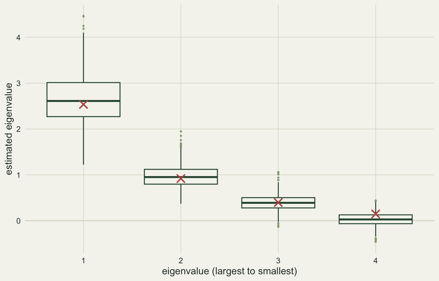

Figure 5.2: Estimated eigenvalues of a four-trait G matrix across simulated parent-offspring studies of 200 families. Crosses mark the true eigenvalues.

The consequence falls on exactly the part of G this chapter has argued matters most. A direction of weak genetic variance is where constraint lives, and it is also where an estimate of G is least reliable and most biased towards looking even weaker than it is. Two things follow for practice. An estimated G should be constrained to be a valid covariance matrix, with no negative variance in any direction, which the restricted maximum likelihood fits of Chapter 7 do by searching only over valid variances and covariances. And a claim that some combination of traits lacks genetic variance needs an interval on that eigenvalue, from resampling or from the posterior of a Bayesian fit, not the point estimate alone.

5.7 What G does not promise

G summarises the additive genetic variation in one population, in one environment, at one time. It changes with allele frequencies, and selection changes allele frequencies; it changes when the environment changes the expression of the genes that build the traits; and it changes under the same selection-induced disequilibrium that reduced the additive variance in Chapter 4, which acts on covariances as well as variances. A G estimated today forecasts the next few generations and not the next few hundred, although the orientation of g_max is often more stable than its size.

Both matrices of this chapter, the P inside the selection gradient and the G inside the response, have now been used as if they were known. P can be estimated from phenotypes alone. G cannot: it has to come from the resemblance between relatives, and that needs a pedigree and a model that can use it. That model is the subject of Part III.

References

Lande R 1979. Evolution 33(1):402-416 (10.1111/j.1558-5646.1979.tb04694.x)

Schluter D 1996. Evolution 50(5):1766-1774 (10.1111/j.1558-5646.1996.tb03563.x)

Hansen TF, Houle D 2008. Journal of Evolutionary Biology 21(5):1201-1219 (10.1111/j.1420-9101.2008.01573.x)

Walsh B, Blows MW 2009. Annual Review of Ecology, Evolution, and Systematics 40:41-59 (10.1146/annurev.ecolsys.110308.120232)

Hill WG, Thompson R 1978. Biometrics 34(3):429-439 (10.2307/2530605)