V_A <- 0.3; V_PE <- 0.2; V_R <- 0.5
V_P <- V_A + V_PE + V_R
h2 <- V_A / V_P
rep_true <- (V_A + V_PE) / V_P
stopifnot(rep_true >= h2)6 Repeatability, the upper limit
Part II ended on a requirement. The additive genetic variance, alone or arranged in G, cannot be read off a set of phenotypes; it shows itself only in the resemblance between relatives, and a model has to be built that can see it there. Before any pedigree is involved, one relative is always available and always perfectly related: the individual itself, measured more than once. The resemblance between repeated measurements of the same animal is the simplest resemblance in quantitative genetics, and the model that describes it, a linear model with a random intercept for each individual, is the skeleton of every model in the rest of this part.
This chapter fits that model, by hand and with nlme, and reads its one ratio, the repeatability, in three ways. It is the upper limit of the heritability. It changes meaning once fixed effects enter the model, and the version that is reported has to be named. And it is the reliability of a single measurement, which is exactly the quantity Chapter 3 needed in order to repair a selection gradient on a noisy trait. The chapter then runs three checks on a repeatability estimate that involve no change in the animals, and ends on what repeated measures cannot do, which is the reason the next chapter needs a pedigree.
6.1 The individual as its own relative
Measure a trait several times on each individual. Each measurement carries the individual’s breeding value a, an environmental effect that the individual keeps across measurements, and a deviation specific to that occasion:
\[ z_{ij} = \mu + a_i + pe_i + e_{ij}, \qquad V_P = V_A + V_{PE} + V_R . \]
The permanent-environment effect pe collects everything that makes an individual consistently different from others for reasons other than the genes it transmits: the conditions it grew up in, a territory it holds for life, non-additive genetic effects, which are fixed within an individual but not passed on in the average way. The residual V_R is the within-individual variance, the part that changes between one measurement and the next. The sum V_A + V_PE is the among-individual variance, written V_I from here on, and the repeatability is its share of the total:
\[ \text{repeatability} = \frac{V_I}{V_P} = \frac{V_A + V_{PE}}{V_A + V_{PE} + V_R} \;\geq\; \frac{V_A}{V_P} = h^2 . \]
The inequality is the reason repeatability matters to a geneticist. V_PE cannot be negative, so the additive part of the among-individual variance can never exceed the whole of it, and a trait with low repeatability cannot be highly heritable (Falconer and Mackay 1996). The book keeps the letter R for the response to selection, so the repeatability is written out in words.
The population simulated below has V_A = 0.30, V_PE = 0.20 and V_R = 0.50, so its heritability is 0.30 and its repeatability 0.50.
6.2 Fitting the random intercept
The random-intercept model treats the individual effects a + pe as draws from a normal distribution with variance V_I and estimates that variance by restricted maximum likelihood (REML), the likelihood of the contrasts left after the fixed effects have been removed. For one random intercept the covariance matrix of the data is block diagonal, its determinant and inverse have closed forms, and the residual variance can be profiled out, so the whole fit is a search along one line. The function below does it for any fixed-effect design matrix X.
reml_fit <- function(y, X, id) {
  pos <- match(id, sort(unique(id))); ni <- tabulate(pos)
  N <- length(y); p <- ncol(X)
  # multiply by the inverse of lambda * ZZ' + I: subtract a shrunken group sum
  minv <- function(v, wt) v - wt[pos] * rowsum(v, pos)[pos, , drop = FALSE]
  core <- function(lg) {
    lam <- exp(lg); wt <- lam / (1 + lam * ni)
    ch <- chol(crossprod(X, minv(X, wt)))
    b <- backsolve(ch, backsolve(ch, crossprod(X, minv(cbind(y), wt)), transpose = TRUE))
    r <- y - drop(X %*% b)
    s2 <- sum(r * minv(cbind(r), wt)) / (N - p)
    list(dev = sum(log(1 + lam * ni)) + 2 * sum(log(diag(ch))) + (N - p) * log(s2),
         s2 = s2, b = drop(b))
  }
  lg <- optimize(function(l) core(l)$dev, c(-12, 8), tol = 1e-10)$minimum
  f <- core(lg)
  list(V_I = exp(lg) * f$s2, V_R = f$s2, b = f$b, fitted = drop(X %*% f$b))
}
rep_of <- function(f) f$V_I / (f$V_I + f$V_R)

sim_rep <- function(V_A, V_PE, V_R, n_ind, k) {
  id <- rep(seq_len(n_ind), each = k)
  a <- rnorm(n_ind, 0, sqrt(V_A)); pe <- rnorm(n_ind, 0, sqrt(V_PE))
  data.frame(id = id, z = (a + pe)[id] + rnorm(n_ind * k, 0, sqrt(V_R)))
}set.seed(606)
n_ind <- 400; k <- 4
d1 <- sim_rep(V_A, V_PE, V_R, n_ind, k)
f_hand <- reml_fit(d1$z, matrix(1, nrow(d1)), d1$id)
f_lme <- lme(z ~ 1, random = ~ 1 | id, data = d1, method = "REML")
vc_lme <- as.numeric(VarCorr(f_lme)[, "Variance"])
stopifnot(abs(f_hand$V_I - vc_lme[1]) < 1e-4, abs(f_hand$V_R - vc_lme[2]) < 1e-4)
# the one-way analysis of variance gives the same answer on balanced data
m_bar <- tapply(d1$z, d1$id, mean)
msb <- k * var(m_bar); msw <- sum((d1$z - m_bar[d1$id])^2) / (n_ind * (k - 1))
stopifnot(abs((msb - msw) / k - f_hand$V_I) < 1e-6, abs(msw - f_hand$V_R) < 1e-6)
rep_hat1 <- rep_of(f_hand)
gap_lme <- max(abs(c(f_hand$V_I, f_hand$V_R) - vc_lme))With 400 individuals measured 4 times each, the hand-coded fit and lme() agree on both variance components to the precision of their optimisers, and on balanced data both agree with the old moment estimator built from the between- and within-individual mean squares, which is the same estimator whenever its answer is positive. The among-individual variance comes out at 0.559 against a true 0.50, the residual at 0.503, and the repeatability at 0.526. The estimate has the precision of 400 individuals, not of 1,600 measurements: a variance among individuals is learned from individuals.
6.3 What repeated measures cannot split
The estimate of 0.526 sits near the repeatability of 0.50 and far from the heritability of 0.30. That is not a failure of the fit. The model has one variance among individuals, and the data contain no information about how that variance divides between genes and permanent environment. The simulation below makes the point with three populations that share the same V_I and divide it in three ways.
splits <- rbind(c(V_A, V_PE), c(0, V_A + V_PE), c(V_A + V_PE, 0))
n_mc <- 200
set.seed(6061)
split_rep <- t(apply(splits, 1, function(s)
  replicate(n_mc, rep_of({d <- sim_rep(s[1], s[2], V_R, n_ind, k)
                          reml_fit(d$z, matrix(1, nrow(d)), d$id)}))))
split_mean <- rowMeans(split_rep); split_sd <- apply(split_rep, 1, sd)
split_h2 <- splits[, 1] / V_P
The three populations have heritabilities of 0.30, 0.00 and 0.50. Over 200 simulated studies each, their mean repeatabilities are 0.498, 0.498 and 0.500, with standard deviations of 0.026, 0.027 and 0.025 across studies. The estimates are indistinguishable because the data are: a normal individual effect with variance V_I has the same distribution whichever of its parts is inherited. Repeated measures on unrelated individuals therefore bound the heritability from above and say nothing about where below the bound it lies. A trait with a repeatability of one half might have a heritability of one half or of zero.
6.4 Adjusted and raw repeatability
A field study rarely fits an intercept alone. Scores change with season, age, time of day or observer, and those effects are fitted as fixed effects. Three ratios then circulate under the one name (Nakagawa and Schielzeth 2010). The raw repeatability ignores the fixed effect and divides the among-individual variance by everything. The adjusted repeatability fits the fixed effect and takes the ratio of the two variance components that remain. The enhanced repeatability keeps the adjusted numerator but puts the variance of the fitted fixed effects, V_F, back into the denominator.
Which one is reported can change the number severalfold, and the direction of the change is set by where the fixed effect sits relative to the individuals. The simulation below uses the same individuals, the same residuals and the same season effect in two field designs. In the first, every individual is measured half its times in each season, so the season contrast lies within individuals. In the second, each individual is measured in one season only, so the contrast lies between them.
V_I_s <- 0.6; V_R_s <- 1.0; b_season <- 2
n_b <- 60; k_b <- 6
rep_s <- V_I_s / (V_I_s + V_R_s)
id_b <- rep(seq_len(n_b), each = k_b)
x_within  <- rep(rep(0:1, each = k_b / 2), times = n_b)
x_between <- rep(rep(0:1, each = n_b / 2), each = k_b)
three_rep <- function(y, x) {
  f0 <- reml_fit(y, matrix(1, length(y)), id_b)
  f1 <- reml_fit(y, cbind(1, x), id_b)
  V_F <- var(f1$fitted)
  c(raw = rep_of(f0), adjusted = rep_of(f1),
    enhanced = f1$V_I / (f1$V_I + f1$V_R + V_F),
    VI_raw = f0$V_I, VR_raw = f0$V_R, VI_adj = f1$V_I, VR_adj = f1$V_R)
}
set.seed(6062)
n_mc2 <- 300
adj <- replicate(n_mc2, {
  base <- rnorm(n_b, 0, sqrt(V_I_s))[id_b] + rnorm(n_b * k_b, 0, sqrt(V_R_s))
  c(three_rep(base + b_season * x_within, x_within),
    three_rep(base + b_season * x_between, x_between))
})
mw <- rowMeans(adj[1:7, ]); mb <- rowMeans(adj[8:14, ])
The true adjusted repeatability is 0.375. Averaged over 300 simulated studies of 60 individuals measured 6 times, the raw repeatability is 0.152 when the season lies within individuals and 0.613 when it lies between them, a factor of 4.04 apart. The adjusted repeatability is 0.370 and 0.369, and the enhanced one 0.228 and 0.228. The adjustment is not what moves between designs. The raw value does.
q_w <- apply(adj[1:3, ], 1, quantile, c(0.025, 0.975))
q_b <- apply(adj[8:10, ], 1, quantile, c(0.025, 0.975))
g3 <- data.frame(
  est = factor(rep(c("raw", "adjusted", "enhanced"), 2),
               levels = c("raw", "adjusted", "enhanced")),
  design = factor(rep(c("season within individuals", "season between individuals"), each = 3),
                  levels = c("season within individuals", "season between individuals")),
  mid = c(mw[1:3], mb[1:3]), lo = c(q_w[1, ], q_b[1, ]), hi = c(q_w[2, ], q_b[2, ]))
ggplot(g3, aes(est, mid, colour = design)) +
  geom_hline(yintercept = rep_s, linetype = "dashed", colour = te_ink) +
  geom_errorbar(aes(ymin = lo, ymax = hi), width = 0.15, linewidth = 0.6,
                position = position_dodge(width = 0.4)) +
  geom_point(size = 3, position = position_dodge(width = 0.4)) +
  scale_colour_manual(values = c(te_forest, te_rust), name = NULL) +
  labs(x = NULL, y = "repeatability") +
  theme_book()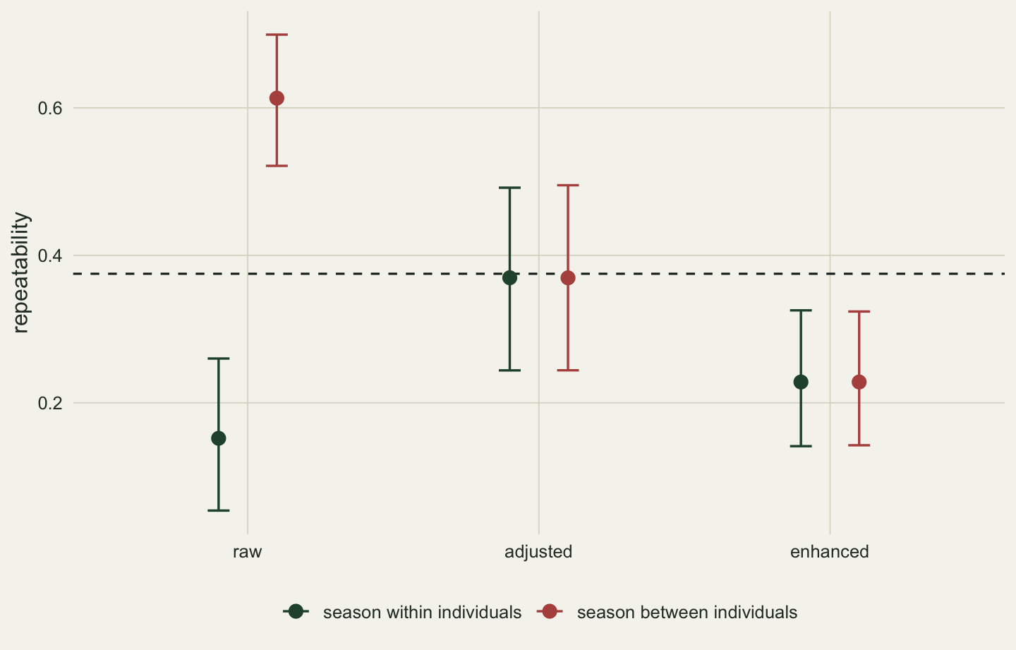
The variance components show where the season went when it was left out. With the season inside each individual’s record, the unadjusted model can only put it in the residual, which rises from 0.999 to 2.192. The among-individual variance also falls, from 0.596 to 0.397, although every individual mean contains both seasons equally: the estimate of V_I is the variance of the means minus a share of the residual, and an inflated residual is over-subtracted. With the season between individuals it is a difference between individuals, and the unadjusted model files it there, raising V_I to 1.609 and leaving the residual at 0.999.
For the upper-limit argument, the adjusted repeatability is the relevant one, and it has to be computed with the same fixed effects as the heritability it is meant to bound. There is one trap in the adjustment itself. A between-individual factor that stands in for something individual, such as the territory an animal holds all its life, removes part of V_PE from the numerator, which is legitimate, and removes part of V_A as well if relatives tend to share territories, which is not. That problem returns with a pedigree in Chapter 9.
6.5 Repeatability as reliability
The same ratio has a second reading. If the within-individual deviations are nothing but noise from the point of view of a later analysis, and the quantity of interest is each individual’s own value, then the repeatability is the reliability of one measurement: the share of its variance that belongs to the individual. Chapter 3 measured what a reliability below one does to selection gradients. Selection on a noisy trait is attenuated, and part of it reappears on a correlated trait that was measured more precisely. It promised that repeated measurements would supply the correction, and the random-intercept model is what supplies it.
The simulation repeats the set-up of Chapter 3, a target trait under selection, measured with the same reliability, and a passenger correlated with it that has no effect on fitness, but now each individual’s target is measured twice. There are two uses for the second measurement. Averaging raises the reliability, to \(k\rho / (1 + (k - 1)\rho)\) for the mean of \(k\) measurements of reliability \(\rho\). And the random-intercept fit estimates V_I, the variance of the individual values themselves, which is what the phenotypic covariance matrix needs on its diagonal before it is inverted. Measurement error adds variance to the noisy trait and leaves its covariances with the other trait and with fitness unchanged, so correcting that single diagonal element corrects the gradient.
set.seed(608)
n_e <- 20000; rel <- 0.6; k_e <- 2
t_lat <- rnorm(n_e)                                    # the individual's own value
pass <- 0.6 * t_lat + sqrt(1 - 0.6^2) * rnorm(n_e)     # passenger, no effect on fitness
id_e <- rep(seq_len(n_e), each = k_e)
meas <- sqrt(rel) * t_lat[id_e] + sqrt(1 - rel) * rnorm(n_e * k_e)
W <- rpois(n_e, exp(0.2 + 0.35 * t_lat)); w <- W / mean(W)
m1   <- meas[seq(1, n_e * k_e, by = k_e)]
mbar <- as.vector(tapply(meas, id_e, mean))
b_true <- coef(lm(w ~ pass + t_lat))[2:3]
b_one  <- coef(lm(w ~ pass + I(m1 / sd(m1))))[2:3]   # per SD of the score
b_mean <- coef(lm(w ~ pass + I(mbar / sd(mbar))))[2:3]   # per SD of the score
se_true <- summary(lm(w ~ pass + t_lat))$coefficients[2:3, 2]
f_e <- reml_fit(meas, matrix(1, length(meas)), id_e)
rel_hat  <- rep_of(f_e)
rel_mean <- k_e * rel_hat / (1 + (k_e - 1) * rel_hat)
P_z <- cov(cbind(pass, mbar)); S_z <- c(cov(pass, w), cov(mbar, w))
P_c <- P_z; P_c[2, 2] <- f_e$V_I                       # the individual values' variance
b_corr <- drop(solve(P_c, S_z)) * c(1, sqrt(f_e$V_I))  # target per SD of its own value
stopifnot(abs(f_e$V_I / (f_e$V_I + f_e$V_R / k_e) - rel_mean) < 1e-12)
With 20,000 individuals, the estimated repeatability of one measurement is 0.599 and that of the mean of 2 is 0.749. With the true individual values in the regression, the gradients are -0.008 on the passenger and 0.366 on the target, with standard errors of about 0.008. A single measurement gives 0.106 and 0.229, the misattribution of Chapter 3. The mean of two measurements, also per standard deviation of the score, gives 0.070 and 0.275: better, and still wrong, because a reliability of 0.75 is not one. The corrected covariance matrix gives -0.006 and 0.363, both within sampling error of the gradients on the true values.
The correction rests on an assumption the arithmetic cannot check. It treats within-individual variation as irrelevant to fitness. For a morphological measurement taken twice with calipers that is true. For a behaviour it may not be: a bird that is bold on the morning a predator arrives is selected for being bold that morning, not on average, and removing its within-individual variation then removes real selection. The repeatability is the reliability of a measurement of the individual’s mean, and whether the mean is the trait selection sees is a biological question.
6.6 How far apart the repeats were
The first check concerns time. The model above holds pe fixed for life. Real permanent-environment effects drift: condition, rank and territory change over months, while an individual’s breeding value does not. A repeatability therefore belongs to the interval between the measurements as much as to the trait (Araya-Ajoy and colleagues 2015). The simulation lets pe follow an autoregressive process, which forgets its past at an exponential rate, and leaves the breeding values fixed.
tau <- 45; n_g <- 1000; n_mc3 <- 100
icc2 <- function(Y) {
  n <- nrow(Y); k <- ncol(Y); rm <- rowMeans(Y)
  msb <- k * sum((rm - mean(rm))^2) / (n - 1); msw <- sum((Y - rm)^2) / (n * (k - 1))
  (msb - msw) / (msb + (k - 1) * msw)
}
gap_rep <- function(gap) {
  rho <- exp(-gap / tau)
  mean(replicate(n_mc3, {
    a <- rnorm(n_g, 0, sqrt(V_A)); pe1 <- rnorm(n_g, 0, sqrt(V_PE))
    pe2 <- rho * pe1 + rnorm(n_g, 0, sqrt(V_PE * (1 - rho^2)))
    icc2(cbind(a + pe1, a + pe2) + matrix(rnorm(2 * n_g, 0, sqrt(V_R)), n_g))
  }))
}
set.seed(6063)
gaps <- c(0.02, 1, 3, 7, 14, 30, 60, 120, 240, 480, 1000)
gap_meas <- vapply(gaps, gap_rep, 0)
gap_pred <- (V_A + V_PE * exp(-gaps / tau)) / V_P
The expected repeatability at a gap t is \((V_A + V_{PE} e^{-t/\tau}) / V_P\), with a timescale \(\tau\) of 45 days. Across 11 gaps from under an hour to nearly three years the measured values never differ from it by more than 0.005. At the shortest gap the repeatability is 0.501; at 30 days it is 0.403; at the longest it is 0.299, the heritability of 0.30 to within simulation noise. The same animals and the same trait give a repeatability anywhere between the two, depending on nothing but the calendar.
gdf <- data.frame(gap = gaps, meas = gap_meas, pred = gap_pred)
ggplot(gdf, aes(gap)) +
  geom_hline(yintercept = c(rep_true, h2), colour = te_sage, linetype = "dotted") +
  annotate("text", x = 1000, y = c(rep_true, h2) + 0.012, hjust = 1, size = 3.4,
           colour = te_body, label = c("short-gap repeatability", "heritability")) +
  geom_line(aes(y = pred), colour = te_forest, linewidth = 0.8) +
  geom_point(aes(y = meas), colour = te_rust, size = 2.4) +
  scale_x_log10(breaks = c(0.02, 1, 7, 30, 180, 1000),
                labels = c("0.02", "1", "7", "30", "180", "1000")) +
  labs(x = "gap between measurements (days, log scale)", y = "repeatability") +
  theme_book()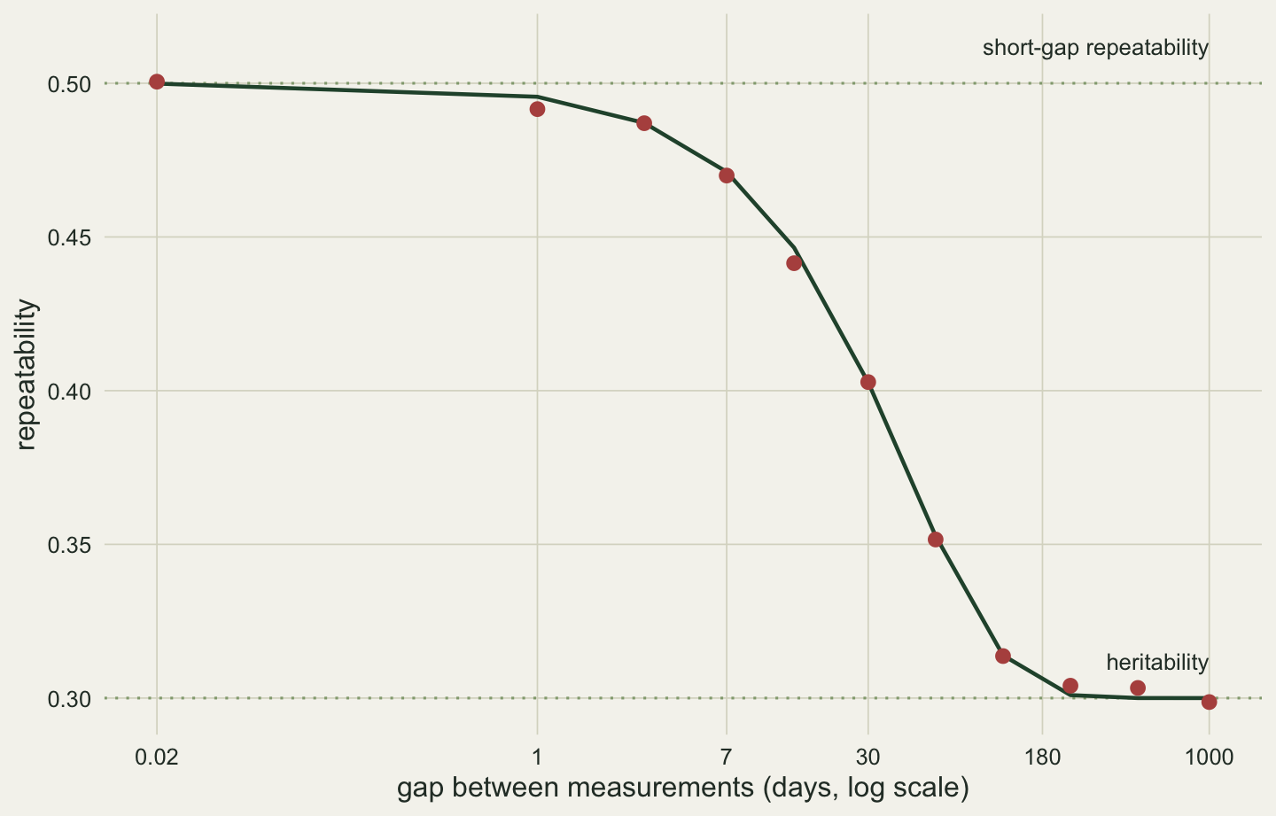
This is a design choice that tightens the upper limit. A long gap lets the drifting part of V_PE decorrelate, and the repeatability falls towards h^2 from above. It reaches it here only because the simulation made all of V_PE drift and all of V_A stay put. In a real population some permanent environment lasts for life, from the conditions of early development for instance, which keeps the long-gap repeatability above h^2; and some additive effects are expressed at one age and not another, which can pull it below h^2. A long-gap repeatability is therefore a tighter bound only when breeding values are stable across the interval, and it is never an estimate. It also means that published repeatabilities are only comparable when they share an interval, which should be reported in the same sentence as the value.
6.7 Who held the stopwatch
The second check concerns observers. When two or more people score the animals and each individual is mostly scored by the same person, any difference between observers is attached to the individual, and the model has no way to tell it apart from V_I.
n_o <- 30; k_o <- 4; m_o <- 6
V_I_o <- 0.30; V_O <- 0.25; V_R_o <- 0.70; share <- 0.85
rep_adj_o <- V_I_o / (V_I_o + V_R_o); rep_unadj_o <- V_I_o / (V_I_o + V_O + V_R_o)
The simulation gives 30 individuals 4 scores each from a pool of 6 observers, with an observer variance of 0.25 against an individual variance of 0.30, and compares a design in which each individual has a main observer with one in which observers are rotated.
id_o <- rep(seq_len(n_o), each = k_o)
icc_long <- function(y) {
  mb <- as.vector(rowsum(y, id_o)) / k_o
  msb <- k_o * sum((mb - mean(mb))^2) / (n_o - 1)
  msw <- sum((y - mb[id_o])^2) / (n_o * (k_o - 1))
  (msb - msw) / (msb + (k_o - 1) * msw)
}
obs_confounded <- function() {
  main <- rep(seq_len(m_o), length.out = n_o)[id_o]
  other <- vapply(main, function(o) sample(setdiff(seq_len(m_o), o), 1), 0)
  ifelse(runif(n_o * k_o) < share, main, other)
}
obs_rotated <- function() as.vector(replicate(n_o, sample(m_o, k_o)))
# REML with crossed random effects for individual and observer
fit_crossed <- function(y, obs) {
  N <- length(y); X <- matrix(1, N)
  K_i <- outer(id_o, id_o, "==") * 1; K_o <- outer(obs, obs, "==") * 1
  core <- function(p) {
    V <- exp(p[1]) * K_i + exp(p[2]) * K_o; diag(V) <- diag(V) + 1
    ch <- chol(V)
    Ly <- backsolve(ch, y, transpose = TRUE); LX <- backsolve(ch, X, transpose = TRUE)
    mu <- sum(LX * Ly) / sum(LX^2); q <- sum((Ly - mu * LX)^2)
    list(dev = 2 * sum(log(diag(ch))) + log(sum(LX^2)) + (N - 1) * log(q / (N - 1)),
         s2 = q / (N - 1))
  }
  op <- optim(c(log(0.4), log(0.3)), function(p) core(p)$dev,
              control = list(reltol = 1e-9, maxit = 500))
  s2 <- core(op$par)$s2
  c(V_I = exp(op$par[1]) * s2, V_O = exp(op$par[2]) * s2, V_R = s2)
}
set.seed(6064)
n_mc4 <- 150
obs_res <- t(replicate(n_mc4, {
  a <- rnorm(n_o, 0, sqrt(V_I_o)); o <- rnorm(m_o, 0, sqrt(V_O))
  e <- rnorm(n_o * k_o, 0, sqrt(V_R_o))
  oc <- obs_confounded(); orot <- obs_rotated()
  yc <- a[id_o] + o[oc] + e; yr <- a[id_o] + o[orot] + e
  fc <- fit_crossed(yc, oc); fr <- fit_crossed(yr, orot)
  c(icc_conf = icc_long(yc), icc_rot = icc_long(yr),
    mod_conf = fc[["V_I"]] / (fc[["V_I"]] + fc[["V_R"]]),
    mod_rot  = fr[["V_I"]] / (fr[["V_I"]] + fr[["V_R"]]),
    VO_hat = fc[["V_O"]])
}))
m_obs <- colMeans(obs_res); se_obs <- apply(obs_res, 2, sd) / sqrt(n_mc4)
The target is the repeatability with observer removed, 0.30; with observer variance left in the denominator it would be 0.24. When each individual has a main observer who scores 85 per cent of its trials, the plain one-way estimate averages 0.366 over 150 studies: the observers’ differences have been counted as differences between animals. Rotating observers removes the inflation and overshoots, to 0.226, because rotation moves the observer variance into the within-individual term and the plain estimate then targets the unadjusted ratio. Fitting observer as a second random effect recovers the target from either design, 0.303 from the confounded one and 0.305 from the rotated one, with Monte Carlo standard errors of about 0.008, and the observer variance is estimated at 0.258 against a true 0.25.
Rotation is a design fix that changes what is being estimated; the model is the fix that keeps it. The same confounding has a genetic version that matters more. If members of a family are scored by the same person, or measured in the same year, the shared nuisance effect makes relatives resemble each other and is counted as additive variance. The animal model of the next chapter inherits every such problem from the random-intercept model, with the pedigree in place of the individual.
6.8 Testing against zero
The last check is the test of whether there is any among-individual variance at all. A variance cannot be negative, and when the true V_I is zero its estimate lands exactly on the boundary in about half of all studies, because the between-individual mean square falls below the within-individual one about half the time. The likelihood-ratio statistic is then exactly zero, and its null distribution is not the chi-squared with one degree of freedom that a routine model comparison assumes. Self and Liang (1987) showed that it is an even mixture of a point mass at zero and that chi-squared.
n_d <- 30; k_d <- 3
df_b <- n_d - 1; df_w <- n_d * (k_d - 1); df_t <- df_b + df_w
# restricted deviance of a balanced one-way design as a function of the repeatability
dev_rep <- function(r, ss) {
  a <- 1 + (k_d - 1) * r; b <- 1 - r
  df_t * log((ss[1] / a + ss[2] / b) / df_t) + df_b * log(a) + df_w * log(b)
}
lrt_zero <- function(Y) {
  rm <- rowMeans(Y)
  ss <- c(k_d * sum((rm - mean(rm))^2), sum((Y - rm)^2))
  msb <- ss[1] / df_b; msw <- ss[2] / df_w
  r_hat <- max(0, (msb - msw) / (msb + (k_d - 1) * msw))
  dev_rep(0, ss) - dev_rep(r_hat, ss)
}
set.seed(6065)
n_null <- 3000; alpha <- 0.05
lrt <- replicate(n_null, lrt_zero(matrix(rnorm(n_d * k_d), n_d)))
at_zero  <- mean(lrt <= 1e-12)
err_chi1 <- mean(lrt > qchisq(1 - alpha, 1))
err_mix  <- mean(lrt > qchisq(1 - 2 * alpha, 1))
In 3,000 simulated studies of 30 individuals measured 3 times, with no among-individual variance at all, the statistic is exactly zero in 52.4 per cent. Against the plain chi-squared threshold of 3.84, the test rejects in 2.6 per cent of studies at a nominal 5 per cent. Against the mixture threshold of 2.71, it rejects in 4.6 per cent. The naive test is conservative by about half, which means it hides real among-individual variance rather than inventing it, and the traits it hides are the weakly repeatable ones. The same boundary applies to every variance component in the chapters that follow, V_A included, and Chapter 10 returns to it.
6.9 From the individual to its relatives
Repeated measures on the same individuals give the among-individual variance cleanly, with a model that fits on a page and agrees with nlme. They give the reliability that corrects a selection analysis for measurement error, and they give an upper limit for the heritability that is only as good as the design behind it: adjusted for the right fixed effects, cleared of observers, and taken over an interval long enough for transient environments to fade. What they cannot give is the split of V_I into V_A and V_PE. The three populations above had heritabilities from zero to the full repeatability and returned the same answer.
The split needs a second kind of resemblance, between individuals that share genes in known proportions and do not share a permanent environment. A parent and its offspring, two half sibs, two cousins: each pair shares a known fraction of its additive variance and, if the design is kind, nothing else. Chapter 7 generalises the random intercept of this chapter to a random effect whose covariance between individuals is set by the pedigree, the additive relationship matrix A, and shows where the permanent-environment intercept built here joins it when records are repeated.
References
Falconer DS, Mackay TFC 1996. Introduction to Quantitative Genetics, 4th ed. Longman. ISBN 978-0582243026
Nakagawa S, Schielzeth H 2010. Biological Reviews 85(4):935-956 (10.1111/j.1469-185X.2010.00141.x)
Araya-Ajoy YG, Mathot KJ, Dingemanse NJ 2015. Methods in Ecology and Evolution 6(12):1462-1473 (10.1111/2041-210X.12430)
Self SG, Liang KY 1987. Journal of the American Statistical Association 82(398):605-610 (10.1080/01621459.1987.10478472)