mendel <- function(x) rbinom(length(x), 1, x / 2)   # one allele from a parent with x copies
make_families <- function(x_par, n_fam, n_sib) {
  s <- sample(length(x_par), n_fam); d <- sample(setdiff(seq_along(x_par), s), n_fam)
  s <- rep(s, each = n_sib); d <- rep(d, each = n_sib)
  data.frame(fam = rep(seq_len(n_fam), each = n_sib), x = mendel(x_par[s]) + mendel(x_par[d]))
}
others_mean <- function(v, fam) (ave(v, fam, FUN = sum) - v) / (ave(v, fam, FUN = length) - 1)
mom <- function(u, v) mean((u - mean(u)) * (v - mean(v)))     # population moments

set.seed(1301)
n_fam <- 5000; n_sib <- 4; c_cost <- 0.2; p0 <- 0.2
fams <- make_families(rbinom(2 * n_fam, 2, p0), n_fam, n_sib)
g <- fams$x / 2
g_oth <- others_mean(g, fams$fam)
r_sib <- mom(g_oth, g) / mom(g, g)
b_demo <- 0.3
w_demo <- 1 - c_cost * g + b_demo * g_oth
split_gap <- mom(w_demo, g) - mom(g, g) * (r_sib * b_demo - c_cost)
stopifnot(abs(split_gap) < 1e-12)
b_star <- c_cost / r_sib13 Relatedness and Hamilton’s rule
Chapter 12 ended on a regression slope. When the fitness of a cooperator depends on the behaviour of its groupmates, the selection covariance splits into a direct part paid by the actor and an indirect part that passes through its partners, and the change in the mean has the sign of \(rb - c\), with \(r\) the slope of the regression of groupmates’ trait on the actor’s own. That slope was large only when groupmates shared founders. The behaviour there was a type copied faithfully from parent to offspring, and the groups were assembled by hand. In a natural population the helping behaviour is carried by genes that segregate at meiosis, the partners are relatives, and how much they share is written in a pedigree. An alarm call costs the caller and protects its neighbours; a helper at the nest raises young that are not its own. Whether a gene for either can spread depends on the same slope, measured now between kin.
This chapter carries the slope into that setting and asks what it is. It shows the rule at work on a gene over many generations, measures relatedness from genotypes without a pedigree, compares the measurement with the relationship matrix A of Chapter 7, and finds that the same pedigree can give it different values depending on the population in which individuals compete. The last section shows that the benefit and the cost of the rule are regression coefficients too.
13.1 The rule for a gene carried by relatives
Consider one locus with an allele that makes its carriers help. Let \(g_i\) be the frequency of the allele within individual \(i\), so zero, one half or one for a diploid, and let the population frequency \(p\) be the mean of \(g\). An offspring’s dose differs from its parent’s by the luck of segregation, which makes a transmission term in the Price equation, but with fair meiosis that term is zero on average, and the expected change in frequency over one generation is the selection term alone,
\[ \bar W \, \Delta p = \operatorname{cov}(W, g) . \]
Let helping be additive. Each individual pays a cost c in proportion to its own dose of the allele and receives a benefit b in proportion to the mean dose among its social partners, written \(g'_i\), so that \(W_i = 1 - c\, g_i + b\, g'_i\). The split of Chapter 12, written for genes, is
\[ \operatorname{cov}(W, g) = -c \operatorname{var}(g) + b \operatorname{cov}(g', g) = \operatorname{var}(g)\,\left(r b - c\right), \qquad r = \frac{\operatorname{cov}(g', g)}{\operatorname{var}(g)} . \]
The allele increases when rb > c, which is Hamilton’s rule (Hamilton 1964a, 1964b), and r in it is the slope of the regression of the partners’ genotype on the actor’s. Hamilton reached the rule through coefficients of relationship computed from pedigrees; Grafen (1985) argued that the regression is what the rule needs, and the rest of the chapter measures what the difference amounts to.
The simulation below builds groups of full siblings from randomly mating parents, gives the allele an additive cost and benefit, and checks the split numerically.
In 5,000 families of 4 siblings, with the allele at a starting frequency of 0.20, the regression of the siblings’ mean genotype on the focal individual’s genotype is 0.499, against the textbook value of one half for full sibs. The split of the covariance holds to the precision of the arithmetic, as it must, since it is algebra. With a cost of 0.20, the rule places the threshold benefit at \(c/r\) = 0.401.
13.2 An altruism allele over many generations
The identity describes one generation of selection. Whether the allele actually spreads also depends on everything the identity leaves out: the random choice of parents, the Mendelian lottery of which allele each offspring receives, and the change in r and in the genetic variance as the frequency moves. The simulation below runs the whole life cycle. Each generation, parents pair at random and produce families of siblings, fitness is computed from each sibling’s own genotype and its siblings’, and the parents of the next generation are drawn from the offspring in proportion to fitness.
run_altruism <- function(b, n_gen, c = c_cost) {
  x_par <- rbinom(2 * n_fam, 2, p0)
  out <- matrix(NA, n_gen, 3, dimnames = list(NULL, c("p", "pred", "r")))
  for (t in seq_len(n_gen)) {
    fm <- make_families(x_par, n_fam, n_sib)
    g <- fm$x / 2; go <- others_mean(g, fm$fam)
    w <- 1 - c * g + b * go
    out[t, ] <- c(mean(g), mom(w, g) / mean(w), mom(go, g) / mom(g, g))
    x_par <- fm$x[sample(nrow(fm), 2 * n_fam, replace = TRUE, prob = w)]
  }
  out
}
set.seed(1302)
n_gen <- 60; n_rep <- 4
b_set <- c(c_cost, 2 * c_cost, 3 * c_cost)            # r b - c below, at and above zero
runs <- lapply(b_set, function(b) replicate(n_rep, run_altruism(b, n_gen), simplify = FALSE))
p_end <- sapply(runs, function(rr) sapply(rr, function(o) o[n_gen, "p"]))
steps <- do.call(rbind, lapply(unlist(runs, recursive = FALSE), function(o)
  data.frame(real = diff(o[, "p"]), pred = o[-n_gen, "pred"])))
step_fit <- coef(lm(real ~ pred, data = steps))
step_cor <- cor(steps$real, steps$pred)
all_gen <- do.call(rbind, unlist(runs, recursive = FALSE))
r_range <- range(all_gen[all_gen[, "p"] > 0.1, "r"])
r_rare  <- range(all_gen[all_gen[, "p"] <= 0.1, "r"])
Three benefits bracket the threshold: 0.20, 0.40 and 0.60, so that \(rb - c\) is negative, zero and positive for full sibs. Each is run 4 times for 60 generations from a frequency of 0.20. Below the threshold the allele falls in every run, to between 0.006 and 0.015. Above it the allele rises in every run, to between 0.734 and 0.779. At the threshold it wanders, ending between 0.157 and 0.238, which is drift in a population of 10,000 breeding adults with no selection to steer it.
traj <- do.call(rbind, lapply(seq_along(b_set), function(k) do.call(rbind, lapply(seq_len(n_rep), function(j)
  data.frame(gen = seq_len(n_gen), p = runs[[k]][[j]][, "p"], run = paste(k, j),
             b = sprintf("b = %.1f", b_set[k]))))))
ggplot(traj, aes(gen, p, group = run, colour = b)) +
  geom_line(linewidth = 0.6) +
  scale_colour_manual(values = setNames(c(te_rust, te_forest, te_gold), sprintf("b = %.1f", b_set)),
                      name = NULL) +
  labs(x = "generation", y = "allele frequency") +
  theme_book()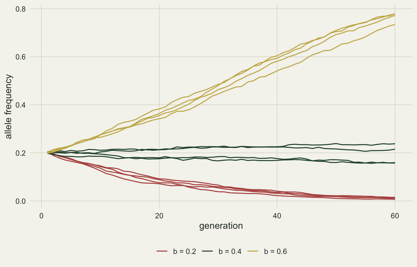
The one-generation prediction also tracks the realised change generation by generation. Across all runs and generations, the regression of the realised change in frequency on the selection term of the Price equation has a slope of 1.044 and an intercept of \(-5.17 \times 10^{-5}\), with a correlation of 0.893 between the two; what the prediction misses is the drift and Mendelian noise of a finite population. The regression relatedness of siblings, recomputed in every generation, stays between 0.463 and 0.529 while the allele frequency is above 0.10, and spreads to between 0.446 and 0.549 once the allele is rare and the regression rests on few carriers. Under random mating the expected value of one half does not depend on the frequency of the allele, which is why the threshold stays put while the population changes around it.
13.4 The population relatedness is measured against
A regression coefficient measures deviations from a mean, and the relevant mean for Hamilton’s rule is not the founders’. The derivation at the start of the chapter used \(\operatorname{cov}(W, g)\), the covariance in the population whose frequency is changing, and an allele spreads by doing better than the other alleles in that population. The reference is the population of competitors: the individuals whose offspring will fill the places that the actor’s offspring might have filled.
Centring every locus on the current generation, rather than the founders, has a precise counterpart for the pedigree. If \(\mathbf C\) is the centring matrix \(\mathbf I - \mathbf 1 \mathbf 1'/n\) for the \(n\) individuals of the current generation, the genotypes centred on their own mean have expected covariance proportional to \(\mathbf C \mathbf A \mathbf C\), so the regression relatedness against the current population is A centred on that population:
\[ \mathbf A_c = \mathbf C \mathbf A \mathbf C, \qquad \operatorname{E}(\hat r_{ij}) \approx \frac{2 A_{c,ij}}{A_{c,ii} + A_{c,jj}} . \]
Centring subtracts the relatedness that every member of the population shares with every other. In a large population that background is small. In a small closed one it is not: its members are related through the few founders they all descend from, and relative to each other that shared ancestry is no longer a deviation from anything.
set.seed(1305)
lg_s <- lg[sample(nrow(lg), 3000), ]
pp <- rbind(
  data.frame(A = lg_s$A, r = lg_s$r_found, pop = "large", ref = "against the founders"),
  data.frame(A = sm$A,   r = sm$r_found,   pop = "small", ref = "against the founders"),
  data.frame(A = lg_s$A, r = lg_s$r_curr,  pop = "large", ref = "against the current population"),
  data.frame(A = sm$A,   r = sm$r_curr,    pop = "small", ref = "against the current population"))
pp$ref <- factor(pp$ref, levels = c("against the founders", "against the current population"))
ggplot(pp, aes(A, r, colour = pop)) +
  geom_abline(slope = 1, intercept = 0, colour = te_ink, linetype = "dashed") +
  geom_point(alpha = 0.25, size = 0.8) +
  facet_wrap(~ ref) +
  scale_colour_manual(values = c(large = te_forest, small = te_gold), name = "population") +
  guides(colour = guide_legend(override.aes = list(alpha = 1, size = 2))) +
  labs(x = "pedigree relatedness A", y = "marker regression relatedness") +
  theme_book()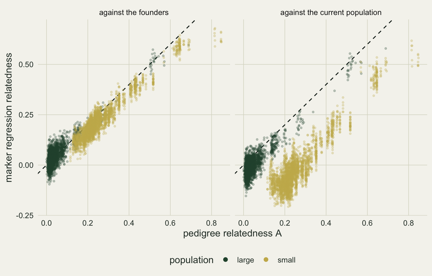
The mean pedigree relatedness between pairs in the last generation is 0.043 in the large population and 0.264 in the small, and the mean inbreeding coefficient is 0.020 and 0.129. The centred prediction matches the marker estimates against the current population with a mean absolute difference of 0.025 in the large population and 0.027 in the small, the same as the scatter of the founder-referenced estimates about their own prediction, 0.025 and 0.025.
The consequence is that the same pedigree relatedness means different things in the two populations. Pairs whose A lies within 0.05 of one half have a mean regression relatedness against their own population of 0.486 in the large population and 0.219 in the small one. Full siblings show the same pattern from the other side. In the small population their mean A is 0.662, above the textbook half because their parents are related, yet their regression relatedness against the population they live in is 0.451. In the large population the corresponding values are 0.528 and 0.492. A pedigree measures relatedness to the founders. Hamilton’s rule needs relatedness relative to the competitors, and a pedigree cannot supply that until it is centred on them.
13.5 Where competition happens
Which population counts as the competitors depends on the ecology, not on the genetics. If the small population of the previous section is one of many demes that exchange offspring freely, so that its young compete with young from everywhere, the competitors are the whole metapopulation. If each deme fills its own breeding places from its own young, the competitors are the deme. The same families, the same genotypes and the same pedigree give two different values of r, and the simulation below checks that each is the right one under its own kind of competition.
set.seed(1304)
n_deme <- 20
demes <- lapply(seq_len(n_deme), function(k) {
  ped <- do.call(sim_pedigree, designs$small)
  A <- build_A(ped$sire, ped$dam); X <- gene_drop(ped, p_f)
  last <- which(ped$gen == max(ped$gen))
  list(A = A[last, last], X = X[last, ], fam = paste(k, ped$sire[last], ped$dam[last]))
})
N <- sapply(demes, function(d) nrow(d$X)); deme <- rep(seq_len(n_deme), N)
G <- do.call(rbind, lapply(demes, `[[`, "X")) / 2
fam <- unlist(lapply(demes, `[[`, "fam"))
G_oth <- apply(G, 2, others_mean, fam = fam)

# pedigree predictions of the sib regression, from A centred on each set of competitors
blocks <- function(f) { M <- matrix(0, sum(N), sum(N)); o <- c(0, cumsum(N))
  for (k in seq_len(n_deme)) { i <- (o[k] + 1):o[k + 1]; M[i, i] <- f(demes[[k]]$A) }; M }
sibs <- outer(fam, fam, "==") & !diag(sum(N)); Wsib <- sibs / rowSums(sibs)
sib_r <- function(M) sum(Wsib * M) / sum(diag(M))       # regression of sib mean on self
A_meta <- blocks(identity)
r_raw    <- sib_r(A_meta)
r_global <- sib_r(centre_A(A_meta))
r_local  <- sib_r(blocks(centre_A))

# selection on each locus as a candidate altruism allele, averaged over loci
cov_cols <- function(U, V) colMeans(U * V) - colMeans(U) * colMeans(V)
sel_global <- function(b) { W <- 1 - c_cost * G + b * G_oth; mean(cov_cols(W, G) / colMeans(W)) }
sel_local <- function(b) { W <- 1 - c_cost * G + b * G_oth
  mean(Reduce(`+`, lapply(seq_len(n_deme), function(k) { i <- deme == k
    N[k] * cov_cols(W[i, ], G[i, ]) / colMeans(W[i, ]) })) / sum(N)) }
b_global <- uniroot(sel_global, c(0.05, 2), tol = 1e-8)$root
b_local  <- uniroot(sel_local,  c(0.05, 2), tol = 1e-8)$root
A metapopulation of 20 demes of the small design, with 1,601 birds in their last generations, is founded from the same gene pool and its demes drift apart for 6 generations. Each locus is treated in turn as a candidate altruism locus with the additive cost and benefit of the first section, siblings as social partners, and a cost of 0.20. Under global competition, fitness is judged against the mean of all demes; under local competition, against the mean of the actor’s own deme, with each deme contributing its fixed share of the next generation. The threshold benefit is found numerically as the value at which selection, averaged over loci, is zero.
The pedigree predicts the sib regression from A alone. Uncentred, it gives 0.577. Centred on the metapopulation it gives 0.573, almost the same, because the pooled population is close to the founders’ gene pool. Centred on each deme it gives 0.469. Under global competition the measured threshold is 0.349, against \(c/r\) = 0.349 from the globally centred pedigree. Under local competition it is 0.426, against 0.426 from the locally centred one. The textbook half would put both at 0.400. Each threshold agrees with the relatedness measured against its own competitors to the third decimal place, and local competition raises the threshold benefit by 22 per cent over global competition.
b_grid <- seq(0.1, 0.7, by = 0.05)
sg <- rbind(data.frame(b = b_grid, sel = vapply(b_grid, sel_global, 0), comp = "global"),
            data.frame(b = b_grid, sel = vapply(b_grid, sel_local, 0),  comp = "local"))
ggplot(sg, aes(b, sel, colour = comp)) +
  geom_hline(yintercept = 0, colour = te_line) +
  geom_vline(xintercept = c_cost / c(r_global, r_local), colour = c(te_forest, te_rust),
             linetype = "dotted") +
  geom_line(linewidth = 0.9) + geom_point(size = 1.6) +
  scale_colour_manual(values = c(global = te_forest, local = te_rust), name = "competition") +
  labs(x = "benefit b", y = "selection on the allele") +
  theme_book()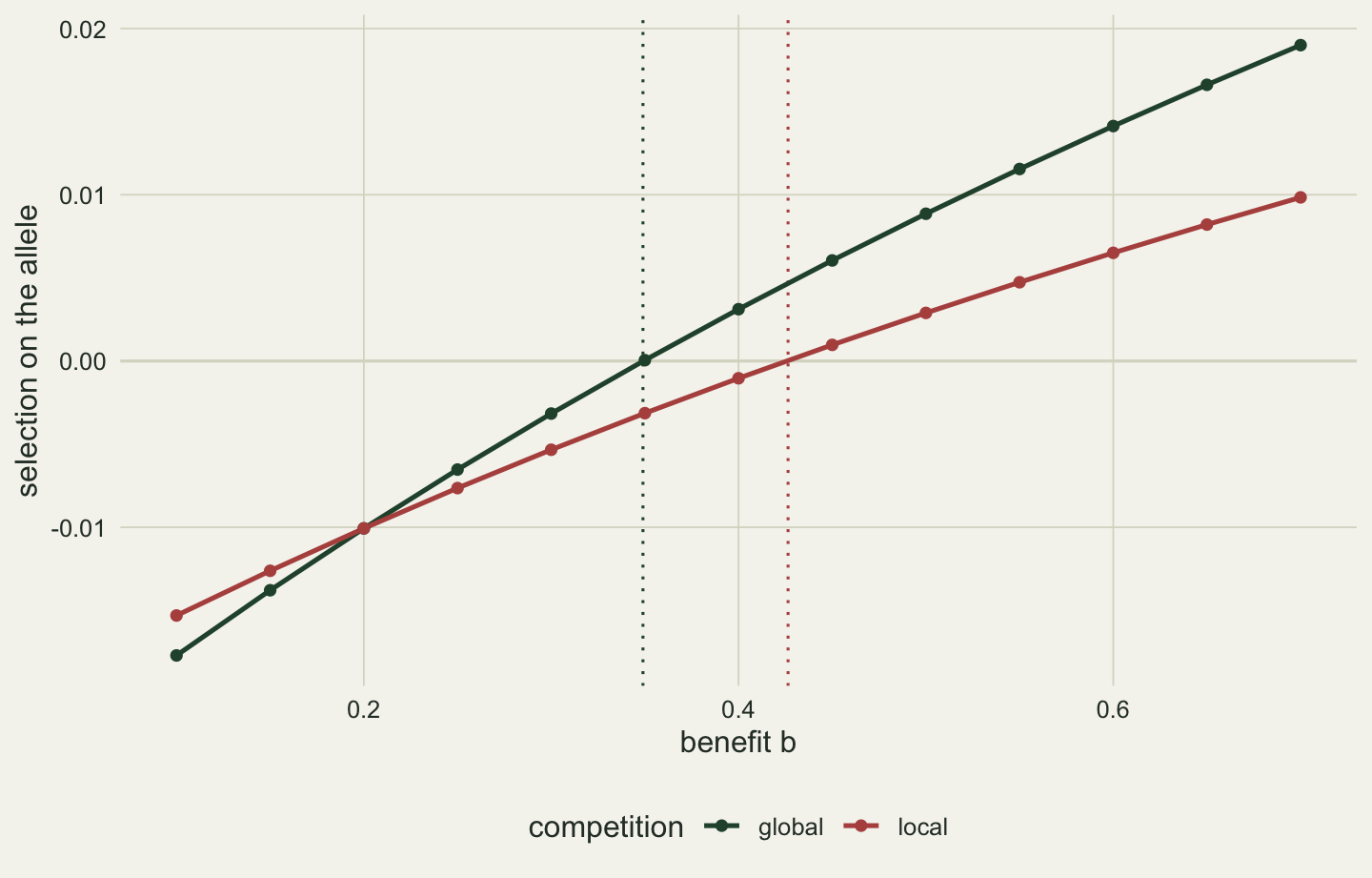
In this accounting local competition makes altruism harder to favour only through relatedness: the benefit a sibling receives is the same in both cases. Chapter 14 writes the same effect the other way, as a benefit and a cost altered by competition. What changes is how far the siblings’ genotypes stand from the mean of the individuals they compete with, and siblings in a small deme stand less far from their deme’s mean than from the metapopulation’s. At the extreme, when the competitors are the group itself, relatedness measured against them is negative whatever the pedigree says; that case, with its consequences for the benefit as well as for r, is one of the checks of Chapter 14.
13.6 Benefit and cost are regression coefficients too
Everything so far assumed that fitness is exactly linear in the actor’s and the partners’ genotypes. Queller (1992) showed that the assumption can be dropped if b and c are redefined. Fit the least squares regression of fitness on the actor’s genotype and the partners’ mean genotype, and call the two partial regression coefficients \(-c\) and \(b\). The residual of a least squares fit is uncorrelated with both predictors, so \(\operatorname{cov}(W, g) = -c \operatorname{var}(g) + b \operatorname{cov}(g', g)\) holds exactly whatever the true shape of fitness. This is the decomposition of Chapter 1, which split a selection differential into direct selection on a trait and indirect selection through the traits correlated with it, with the partners’ genotype in the place of the correlated trait. There the partial coefficients were selection gradients; here they are the cost and the benefit, and the regression of one predictor on the other is relatedness. Hamilton’s rule with all three as regression coefficients is an identity.
What the identity costs shows once fitness is not linear. In the simulation below the benefit saturates: a few helping siblings give most of what many would give.
sat <- function(x, k = 4) (1 - exp(-k * x)) / (1 - exp(-k))  # saturating benefit, sat(1) = 1
b_nom <- 0.5
queller <- function(p, n_f = 20000) {
  fm <- make_families(rbinom(2 * n_f, 2, p), n_f, n_sib)
  g <- fm$x / 2; go <- others_mean(g, fm$fam)
  w <- 1 - c_cost * g + b_nom * sat(go)
  co <- coef(lm(w ~ g + go))
  r <- mom(go, g) / mom(g, g)
  gap <- mom(w, g) - (co[["g"]] * mom(g, g) + co[["go"]] * mom(go, g))
  c(p = mean(g), b = co[["go"]], c = -co[["g"]], r = r, rule = r * co[["go"]] + co[["g"]],
    sel = mom(w, g) / mean(w), gap = gap)
}
set.seed(1306)
p_set <- c(0.1, 0.5, 0.9)
qt <- t(sapply(p_set, queller))
stopifnot(all(abs(qt[, "gap"]) < 1e-12), all(sign(qt[, "rule"]) == sign(qt[, "sel"])))
The nominal benefit, for a sibling whose partners all carry two copies of the allele, is 0.50 and the cost 0.20, so the naive rule with siblings at one half says the allele always spreads. The regression coefficients say something else. At an allele frequency of 0.10 the fitted benefit is 0.884 and the fitted cost 0.156; at 0.50 they are 0.435 and 0.197; at 0.90 they are 0.151 and 0.206. Relatedness stays near one half throughout, between 0.493 and 0.506. The quantity \(rb - c\) is 0.292, 0.018 and -0.130 at the three frequencies, and its sign matches the sign of selection each time, as the identity guarantees. The allele is favoured when rare and opposed when common, so selection changes sign at some intermediate frequency and holds the allele there, which the naive rule with the nominal benefit does not predict.
When helping is common, most individuals already have helping partners, and one more helping sibling adds little; the fitted benefit is the slope of fitness at the partner genotypes the population actually contains. That is the same dependence that made the selection gradients of Part I properties of a population as well as of a fitness function. The rule in regression form gets the direction of selection right in the population where the coefficients were measured, and it carries over to another population only when fitness is linear. Chapter 14 takes the opposite case, a benefit that grows when partners help, and measures how the fitted benefit and cost, and with them the sign of selection, move with the frequency of the allele.
13.7 From the rule to its checks
Relatedness has turned out to be one quantity seen from three places. It is the regression of partners’ genotypes on the actor’s, which is what the Price equation needs. Taken against the founders of a pedigree, its expected value is the relationship matrix A of the animal model, scaled by the actors’ inbreeding. Taken against the population in which selection acts, it is A centred on that population, and that is the version Hamilton’s rule uses. The same sibling families carry a relatedness of 0.573 against their metapopulation and 0.469 against their own deme, and each value predicts the threshold benefit under its own kind of competition. The benefit and the cost of the rule are regression coefficients as well, so the rule holds as an identity at the price of describing one population at one moment.
An identity cannot be wrong, but an analysis that uses it can be. Every quantity in it has to be measured against the right population, with the right partners, on fitness that includes the right competitors, and the textbook numbers for relatedness, benefit and cost are each a tempting shortcut. Chapter 14 takes the rule to the places where those shortcuts fail: payoffs that are not additive, relatives who compete with each other, help that does not reach the kin it is supposed to reach, and a pedigree whose fathers are not all the real fathers.
References
Hamilton WD 1964a. Journal of Theoretical Biology 7(1):1-16 (10.1016/0022-5193(64)90038-4)
Hamilton WD 1964b. Journal of Theoretical Biology 7(1):17-52 (10.1016/0022-5193(64)90039-6)
Grafen A 1985. Oxford Surveys in Evolutionary Biology 2:28-90
Queller DC 1992. Evolution 46(2):376-380 (10.1111/j.1558-5646.1992.tb02045.x)
Queller DC, Goodnight KF 1989. Evolution 43(2):258-275 (10.1111/j.1558-5646.1989.tb04226.x)