amat <- function(sire, dam) {
  n <- length(sire)
  A <- matrix(0, n, n)
  for (i in seq_len(n)) {
    s <- sire[i]; d <- dam[i]
    if (i > 1L) {
      idx <- seq_len(i - 1L)
      v <- 0.5 * ((if (s > 0L) A[idx, s] else 0) + (if (d > 0L) A[idx, d] else 0))
      A[idx, i] <- v; A[i, idx] <- v
    }
    A[i, i] <- 1 + if (s > 0L && d > 0L) 0.5 * A[s, d] else 0   # inbreeding
  }
  A
}
# founders 1, 2, 3, 7, 8; 4 and 5 full sibs; 6 a paternal half sib of both;
# 9 and 10 the offspring of the two full sibs with unrelated mates
demo <- amat(c(0, 0, 0, 1, 1, 1, 0, 0, 4, 5), c(0, 0, 0, 2, 2, 3, 0, 0, 7, 8))
r_po <- demo[1, 4]; r_fs <- demo[4, 5]; r_hs <- demo[4, 6]; r_fc <- demo[9, 10]
stopifnot(abs(r_po - 1/2) < 1e-12, abs(r_fs - 1/2) < 1e-12, abs(r_hs - 1/4) < 1e-12,
abs(r_fc - 1/8) < 1e-12, demo[1, 3] == 0, all(diag(demo) == 1))8 Which relatives carry the information
Chapter 7 ended on a spread. Fresh pedigrees of one nest-box design, each analysed by the same REML fit, returned heritabilities spread so widely that two honest studies of the same population could disagree without either being wrong, and a pedigree of a few hundred birds supported a statement about wing length and not much more. The obvious response is to ask for more birds. This chapter argues that the obvious response is the wrong first question. A pedigree does not inform an estimate of V_A one animal at a time. It informs it through comparisons between animals whose expected resemblance differs, and animals with no known relatives offer no such comparison, however many of them are measured.
The argument is made by holding the number of phenotyped animals fixed and changing only how they are related. Four pedigrees carry the same animals: one with no relationships at all, one of full-sib families, one of paternal half-sib families and one that runs through several generations of random mating. Each is simulated many times and fitted by restricted maximum likelihood, so that precision is measured rather than argued. The expected results appear, and so does one that is not expected: the most natural summary of how much relatedness a pedigree contains ranks two of the designs in the wrong order. The quantity that ranks them correctly comes from the eigenvalues of A, and it can be computed before a single animal is caught.
8.1 Four arrangements of the same animals
The relationship matrix is built by the recursion of Chapter 7, which Henderson (1976) set out: parents before offspring, each new off-diagonal entry the mean of the earlier animal’s relationships with the two parents, and each diagonal entry one plus half the relationship between the parents. The version below fills a whole column at a time instead of looping over earlier animals, and it is checked on a small pedigree of known shape before it is used on anything larger.
The check pedigree has a parent and offspring at 0.5, full sibs at 0.5, a half sib at 0.25, first cousins at 0.125, unrelated founders at zero and nobody inbred. With that settled, the four designs.
ped_unrelated <- function(n) list(sire = rep(0L, n), dam = rep(0L, n), pheno = seq_len(n))
ped_fullsib <- function(nfam, ksib) {
  np <- 2L * nfam                                    # unphenotyped parents first
  list(sire = c(rep(0L, np), rep(seq(1L, np, by = 2L), each = ksib)),
       dam  = c(rep(0L, np), rep(seq(2L, np, by = 2L), each = ksib)),
       pheno = np + seq_len(nfam * ksib))
}
ped_halfsib <- function(nsire, ndam) {                # one offspring per dam
  nd <- nsire * ndam; np <- nsire + nd
  list(sire = c(rep(0L, np), rep(seq_len(nsire), each = ndam)),
       dam  = c(rep(0L, np), nsire + seq_len(nd)),
       pheno = np + seq_len(nd))
}
ped_deep <- function(ngen, per) {                     # random mating, all phenotyped
  sire <- dam <- rep(0L, per); half <- per / 2
  for (g in 2:ngen) {
    prev <- (g - 2L) * per + seq_len(per)
    sire <- c(sire, sample(prev[seq_len(half)], per, replace = TRUE))
    dam  <- c(dam, sample(prev[half + seq_len(half)], per, replace = TRUE))
  }
  list(sire = sire, dam = dam, pheno = seq_len(ngen * per))
}
sub_a <- function(ped) amat(ped$sire, ped$dam)[ped$pheno, ped$pheno]

n_total <- 480
n_fam <- 120; k_sib <- 4          # full sib families
n_sire <- 24; n_dam <- 20         # half sib sire groups
n_gen <- 6; per_gen <- 80         # deep pedigree
set.seed(808)
peds <- list(unrelated = ped_unrelated(n_total), fullsib = ped_fullsib(n_fam, k_sib),
             halfsib = ped_halfsib(n_sire, n_dam), deep = ped_deep(n_gen, per_gen))
amats <- lapply(peds, sub_a)
stopifnot(all(sapply(amats, nrow) == n_total))
ped_rows <- sapply(peds, function(p) length(p$sire))
F_deep <- mean(diag(amats$deep)) - 1                 # mean inbreeding in the deep design
Every design has 480 phenotyped animals. The unrelated design is 480 founders and nothing else. The full-sib design is 120 families of 4, each from its own unrelated pair of parents. The half-sib design mates each of 24 sires to 20 dams and keeps one offspring per dam, so that every pair within a sire group shares a father and no pair shares both parents. In these two the parents are in the pedigree but carry no phenotype, which is how a breeding experiment usually ends up, and the pedigrees have 720 and 984 rows. The deep design is 6 generations of 80 animals, each generation bred from parents drawn at random from the one before, with every animal measured. Random mating in so small a population makes relatives breed with relatives now and then, and the mean inbreeding coefficient reaches 0.9 per cent: enough to be visible on the diagonal of A, too little to matter for what follows.
off <- lapply(amats, function(A) A[upper.tri(A)])
n_pairs <- choose(n_total, 2)
n_linked <- sapply(off, function(x) sum(x > 1e-9))
sum_sq <- sapply(off, function(x) sum(x^2))
deep_weak <- sum(off$deep > 1e-9 & off$deep < r_fc - 1e-9)
deep_close <- sum(off$deep >= r_fs - 1e-9)
stopifnot(n_linked[["unrelated"]] == 0,
          n_linked[["fullsib"]] == n_fam * choose(k_sib, 2),
          n_linked[["halfsib"]] == n_sire * choose(n_dam, 2))
pair_ratio <- n_linked[["halfsib"]] / n_linked[["fullsib"]]
weight_ratio <- (r_fs / r_hs)^2
excerpt <- list(unrelated = 1:60, fullsib = 1:60, halfsib = 1:60,
deep = as.vector(sapply(0:5, function(g) g * per_gen + 1:10)))
design_labs <- c(unrelated = "unrelated", fullsib = "full sib", halfsib = "half sib", deep = "deep")
heat <- do.call(rbind, lapply(names(amats), function(nm) {
sub <- amats[[nm]][excerpt[[nm]], excerpt[[nm]]]; diag(sub) <- NA
gr <- expand.grid(i = 1:60, j = 1:60)
data.frame(gr, r = as.vector(sub), design = design_labs[[nm]])
}))
heat$design <- factor(heat$design, levels = design_labs)
ggplot(heat, aes(j, i, fill = r)) +
geom_raster() +
facet_wrap(~ design, nrow = 1) +
scale_y_reverse(expand = c(0, 0)) + scale_x_continuous(expand = c(0, 0)) +
scale_fill_gradientn(colours = c(te_line, te_sage, te_forest, te_ink),
na.value = te_paper, name = "relatedness") +
coord_fixed() + labs(x = NULL, y = NULL) +
theme_book() +
theme(axis.text = element_blank(), panel.grid = element_blank(),
panel.border = element_rect(colour = te_body, fill = NA, linewidth = 0.4))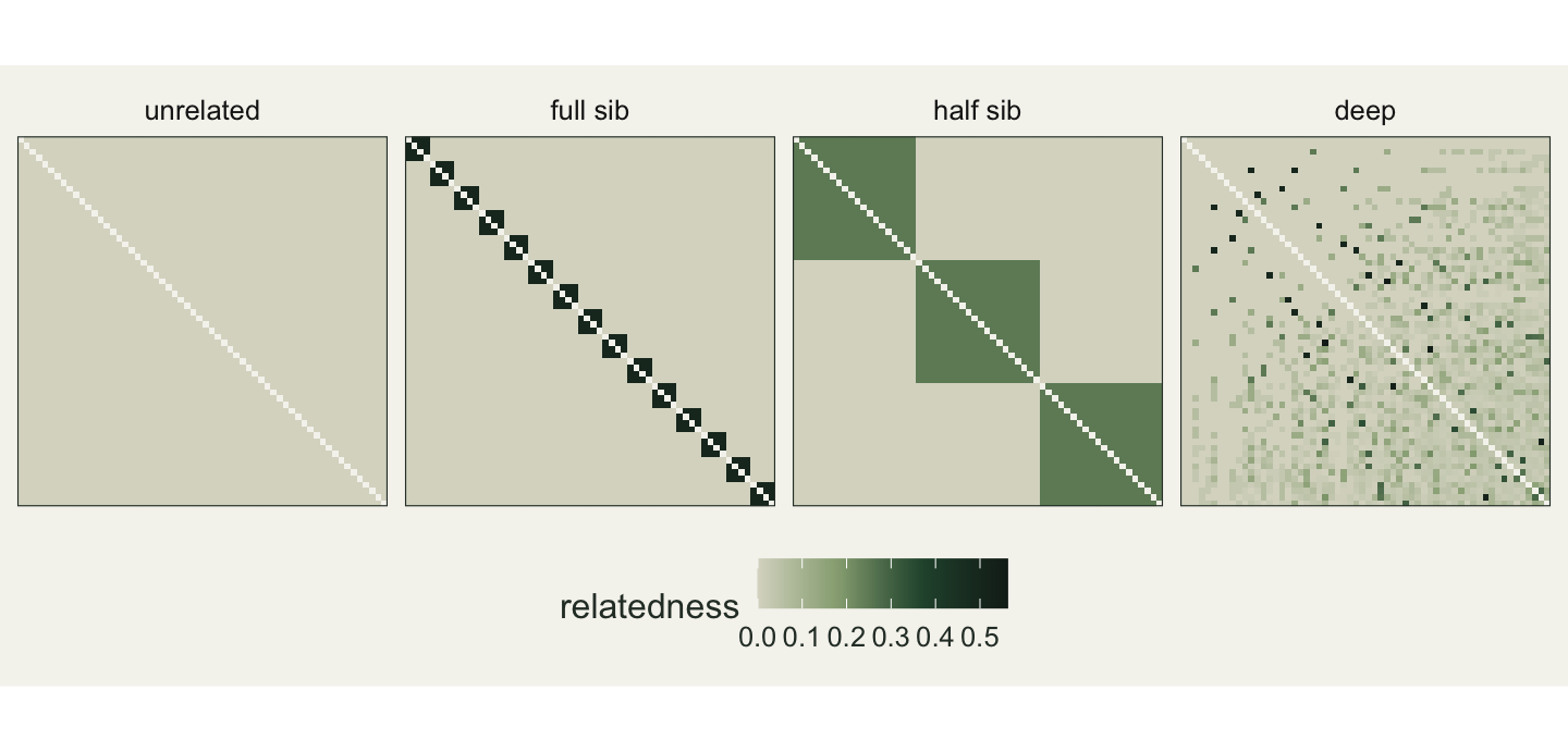
The figure above shows the four structures on a sixty-animal excerpt. The full-sib design is a chain of small dark blocks, the half-sib design a few large, lighter ones, and the deep design has no blocks at all: a scatter of strong links where parents and offspring or full sibs happen to fall near each other in the ordering, over a faint background that thickens in the later generations as everybody becomes a little related to everybody else.
Counted over all 114,960 pairs, the unrelated design has no related pair. The full-sib design has 720, all at 0.5, and the half-sib design 4,560, all at 0.25. The deep design has 52,725 related pairs of every strength: 820 at 0.5 or above, the strongest at 0.66 because some parents are themselves related, and 44,782 weaker than first cousins.
A natural way to judge these designs is to add up the squares of the off-diagonal entries of A. The squaring has a respectable motive, since a squared relatedness is what enters the information about a variance ratio when the ratio is small, and the result looks like a measure of how much comparison a pedigree offers. It gives zero for the unrelated design, 180 for full sibs, 285 for half sibs and 552 for the deep pedigree. On that ranking the half-sib design beats the full-sib design. It has 6.33 times as many related pairs, each down-weighted by a factor of 4 by the squaring, and the count wins by a factor of 1.58. That is a prediction, and the rest of the chapter measures it.
8.2 A likelihood that runs on eigenvalues
The model is the animal model of Chapter 7 with an intercept as the only fixed effect. For a precision study it pays to parameterise it by the heritability itself. Writing V_P for V_A + V_R, the phenotypes have covariance
\[ \mathbf V = V_P \mathbf H, \qquad \mathbf H = h^2 \mathbf A + (1 - h^2)\mathbf I , \]
and if \(\mathbf A = \mathbf U \mathbf D \mathbf U'\) then \(\mathbf H = \mathbf U\left(h^2 \mathbf D + (1 - h^2)\mathbf I\right)\mathbf U'\). The rotated phenotypes \(\mathbf U'\mathbf y\) are independent, the \(i\)th with variance \(V_P(h^2 d_i + 1 - h^2)\). The total variance drops out of the restricted likelihood in closed form, which leaves a one-dimensional search over h^2 on the interval from zero to one, with the same lower boundary Chapter 7 built into its search and an upper one added at one. Each replicate then costs arithmetic on a vector of 480 numbers, and replicates can be drawn directly in the rotated space.
reml_prep <- function(A) {
  eg <- eigen(A, symmetric = TRUE)
  list(d = pmax(eg$values, 1e-9), n = nrow(A), U = eg$vectors,
       xt = as.numeric(crossprod(eg$vectors, rep(1, nrow(A)))))
}
# REML deviance for h2 with the total variance profiled out
dev_h2 <- function(h2, st, yt) {
  lam <- h2 * st$d + (1 - h2); w <- 1 / lam
  xhx <- sum(st$xt^2 * w); xhy <- sum(st$xt * yt * w); yhy <- sum(yt^2 * w)
  nm <- st$n - 1; ypy <- yhy - xhy^2 / xhx
  nm * log(ypy / nm) + sum(log(lam)) + log(xhx) + nm
}
h2_grid <- seq(0, 0.999, length.out = 61)
fit_h2 <- function(st, yt) {
  dv <- vapply(h2_grid, dev_h2, 0, st = st, yt = yt); k <- which.min(dv)
  op <- optimize(dev_h2, h2_grid[c(max(1, k - 1), min(61, k + 1))], st = st, yt = yt, tol = 1e-7)
  if (op$objective < dv[k]) op$minimum else h2_grid[k]
}
preps <- lapply(amats, reml_prep)

# the rotated deviance must equal the same deviance computed with full matrices
V_A <- 0.4; V_R <- 0.6; h2_true <- V_A / (V_A + V_R)
set.seed(8081)
A_hs <- amats$halfsib
y <- 3 + drop(crossprod(chol(A_hs), rnorm(n_total))) * sqrt(V_A) + rnorm(n_total, 0, sqrt(V_R))
dev_full <- function(h2, A, y) {
  H <- h2 * A + (1 - h2) * diag(nrow(A)); Hi <- solve(H); one <- rep(1, nrow(A))
  xhx <- sum(Hi); nm <- nrow(A) - 1
  ypy <- drop(t(y) %*% Hi %*% y) - drop(t(one) %*% Hi %*% y)^2 / xhx
  nm * log(ypy / nm) + as.numeric(determinant(H)$modulus) + log(xhx) + nm
}
yt_hs <- drop(crossprod(preps$halfsib$U, y))
dev_gap <- max(abs(sapply(c(0.1, 0.4, 0.8), function(h)
  dev_h2(h, preps$halfsib, yt_hs) - dev_full(h, A_hs, y))))
stopifnot(dev_gap < 1e-6)

eig <- lapply(preps, function(s) s$d)
n_above <- sapply(eig, function(d) sum(d > 1 + 1e-6))
n_below <- sapply(eig, function(d) sum(d < 1 - 1e-6))
stopifnot(all(abs(eig$unrelated - 1) < 1e-9),
          n_above[["fullsib"]] == n_fam, n_above[["halfsib"]] == n_sire)
sim_yt <- function(st, va, vr) rnorm(st$n, 0, sqrt(va * st$d + vr))   # U'y drawn directly
The chunk compares the rotated deviance with the same deviance computed from full matrices on a simulated half-sib data set, at three values of h^2, and they agree to the precision of the arithmetic. The true values throughout are V_A = 0.40 and V_R = 0.60, so h^2 = 0.40.
The eigenvalues deserve a closer look, because the rest of the chapter is written in them. In the unrelated design A is the identity and every eigenvalue is one. In the full-sib design there are 120 eigenvalues of 2.5, one per family, and 360 of 0.5. In the half-sib design there are 24 of 5.75, one per sire, and 456 of 0.75. The deep design has a continuous spectrum from 0.106 to 17.93, with 128 eigenvalues above one and 338 below.
Each eigenvector is a contrast among the phenotypes. The large eigenvalues belong to contrasts between families, differences in family means; the small ones belong to contrasts within families, differences between relatives. The variance of a contrast is \(V_P(h^2 d_i + 1 - h^2)\), so a contrast with \(d_i = 1\) has variance \(V_P\) whatever the heritability, and tells the likelihood nothing about it. The further an eigenvalue sits from one, in either direction, the more the variance of its contrast depends on h^2. That sentence is the whole of the chapter in compressed form.
8.3 A pedigree without relatives
The unrelated design is the limiting case. With A equal to the identity, \(\mathbf H = h^2\mathbf I + (1 - h^2)\mathbf I = \mathbf I\) for every value of h^2, and the likelihood cannot depend on the parameter.
set.seed(8082)
prof_unrel <- vapply(h2_grid, dev_h2, 0, st = preps$unrelated,
                     yt = sim_yt(preps$unrelated, V_A, V_R))
prof_half  <- vapply(h2_grid, dev_h2, 0, st = preps$halfsib,
                     yt = sim_yt(preps$halfsib, V_A, V_R))
stopifnot(diff(range(prof_unrel)) < 1e-8)
n_rep <- 2000
unrel_reps <- replicate(n_rep, fit_h2(preps$unrelated, sim_yt(preps$unrelated, V_A, V_R)))
Across the grid of 61 values the deviance of an unrelated data set does not move, to the precision of the arithmetic, while a half-sib data set of the same size moves its deviance by 19.21 over the same interval. The difference is not one of degree. The phenotypes of unrelated animals have the same distribution whether the trait is entirely additive or entirely environmental, so no amount of them can tell the two apart.
What a fitting routine does with a flat likelihood is the dangerous part, because it does not announce it. The grid search here finds a tie across every point and which.min returns the first, so all 2,000 replicates return the same estimate, 0, with a standard deviation of 0. A spread of zero reads like perfect precision and is the absence of any information. A different optimiser would return its starting value with the same consistency; a package that reports a standard error would report an enormous one or fail to converge, which is the honest outcome. A heritability reported from animals with no known relationships, whether through a pedigree or through markers, comes from the starting value, the prior or the boundary, and not from the data.
8.4 Same animals, different precision
The three informative designs are each fitted to 2,000 replicate data sets.
set.seed(8083)
reps <- lapply(preps[c("fullsib", "halfsib", "deep")], function(st)
  replicate(n_rep, fit_h2(st, sim_yt(st, V_A, V_R))))
sd_h2 <- sapply(reps, sd)
bias  <- sapply(reps, mean) - h2_true
at0   <- sapply(reps, function(x) mean(x < 1e-3))
mc_se <- sd_h2 / sqrt(2 * (n_rep - 1))     # Monte Carlo standard error of a standard deviation
q90   <- sapply(reps, quantile, c(0.05, 0.95))
w90   <- q90[2, ] - q90[1, ]
All three are close to unbiased: the mean estimates lie within 0.004 of the truth, small against the spreads, and no more than 0.05 per cent of any design’s replicates stop at zero. The designs can therefore be compared on spread alone. The standard deviations of the estimates are 0.096 for full sibs, 0.158 for half sibs and 0.080 for the deep pedigree, each with a Monte Carlo standard error of 0.002 or less.
dens <- do.call(rbind, lapply(names(reps), function(nm) {
  dn <- density(reps[[nm]], from = 0, to = 1, n = 512)
  data.frame(h2 = dn$x, dens = dn$y, design = design_labs[[nm]])
}))
dens$design <- factor(dens$design, levels = design_labs[-1])
ggplot(dens, aes(h2, dens, colour = design)) +
  geom_vline(xintercept = h2_true, colour = te_body, linetype = "dashed") +
  geom_line(linewidth = 1) +
  scale_colour_manual(values = c("full sib" = te_rust, "half sib" = te_gold, "deep" = te_forest),
                      name = NULL) +
  labs(x = "estimated heritability", y = "density") +
  theme_book()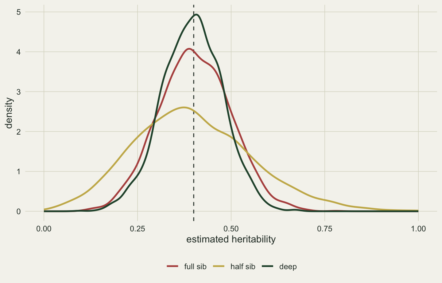
Two findings sit in those numbers. The expected one is that the deep pedigree is the most precise at a fixed sample size, with a standard deviation 1.97 times smaller than the half-sib design’s and 1.19 times smaller than the full-sib design’s. The unexpected one is that the full-sib design beats the half-sib design, by a factor of 1.65 in standard deviation, when the sum of squared relatedness predicted the reverse by a factor of 1.26.
In the terms of a results section, the central ninety per cent of half-sib estimates runs from 0.157 to 0.675, an interval 0.52 wide that cannot tell a trait with a third of its variance additive from one with two thirds. The same animals arranged as a deep pedigree give an interval from 0.263 to 0.527, 0.26 wide. The number of animals measured is identical; the question the study can answer is not.
8.6 Sample size and the zero boundary
The information calculation is a large-sample device, and its reach is worth testing. Holding the half-sib structure at 20 dams per sire and halving the number of sires three times gives four sample sizes, the largest being the design already fitted.
n_sires <- c(3, 6, 12)               # the fourth size, 24 sires, is the main half sib run
size_n <- c(n_sires, n_sire) * n_dam
size_preps <- lapply(n_sires, function(s) reml_prep(sub_a(ped_halfsib(s, n_dam))))
set.seed(8084)
size_reps <- c(lapply(size_preps, function(st) replicate(n_rep, fit_h2(st, sim_yt(st, V_A, V_R)))),
               list(reps$halfsib))
size_sd   <- sapply(size_reps, sd)
size_pred <- c(sapply(size_preps, asym_sd, h2 = h2_true), pred_sd[["halfsib"]])
size_at0  <- sapply(size_reps, function(x) mean(x < 1e-3))
size_at1  <- sapply(size_reps, function(x) mean(x > 0.99))
size_bias <- sapply(size_reps, mean) - h2_true
size_rmse <- sapply(size_reps, function(x) sqrt(mean((x - h2_true)^2)))
size_ratio <- size_pred / size_sd
slope_meas <- unname(coef(lm(log(size_sd) ~ log(size_n)))[2])
slope_pred <- unname(coef(lm(log(size_pred) ~ log(size_n)))[2])
stopifnot(abs(slope_pred + 0.5) < 1e-6)   # information is linear in the number of sires
The information is linear in the number of sires, so the predicted standard deviation falls exactly as one over the square root of the sample size, a slope of -0.50 on log scales. The measured slope across 60 to 480 offspring is -0.380, shallower than that. The cause is the parameter space. At 60 offspring 26 per cent of replicates stop at zero and 11 per cent at the upper end of the interval, and an estimator piled against its walls cannot spread as far as the theory allows: the prediction overstates the measured spread by a factor of 1.26 there, 1.10 at 120, and is within a few per cent from 240 upwards, where under 2 per cent of estimates reach zero.
A spread narrower than the prediction at small samples is no gift. The estimates at 60 offspring are biased downwards by 0.057, and their root mean squared error of 0.353 against 0.158 at 480 says what the design is worth. For a design that leaves many estimates on a boundary the large-sample formula is the wrong tool, and the reliable answer is a simulation of the kind this chapter runs.
cells <- c("FS480", "HS480", "DEEP480", paste0("HS", size_n[1:3]))
meas <- c(sd_h2, size_sd[1:3])
ss <- c(sum_sq[-1], sapply(n_sires, function(s) {
  A <- sub_a(ped_halfsib(s, n_dam)); sum(A[upper.tri(A)]^2) }))
pr <- rbind(data.frame(cell = cells, measured = meas, predicted = 1 / sqrt(ss),
                       rule = "sum of squared relatedness"),
            data.frame(cell = cells, measured = meas, predicted = c(pred_sd, size_pred[1:3]),
                       rule = "REML information"))
pr$rule <- factor(pr$rule, levels = c("sum of squared relatedness", "REML information"))
ggplot(pr, aes(predicted, measured)) +
  geom_abline(slope = 1, intercept = 0, colour = te_sage, linetype = "dashed") +
  geom_point(colour = te_rust, size = 2.4) +
  geom_text(aes(label = cell), size = 3, colour = te_ink, vjust = -0.9) +
  facet_wrap(~ rule) +
  scale_x_log10(limits = c(0.025, 0.9)) + scale_y_log10(limits = c(0.05, 0.7)) +
  labs(x = "predicted sd of heritability", y = "measured sd of heritability") +
  theme_book()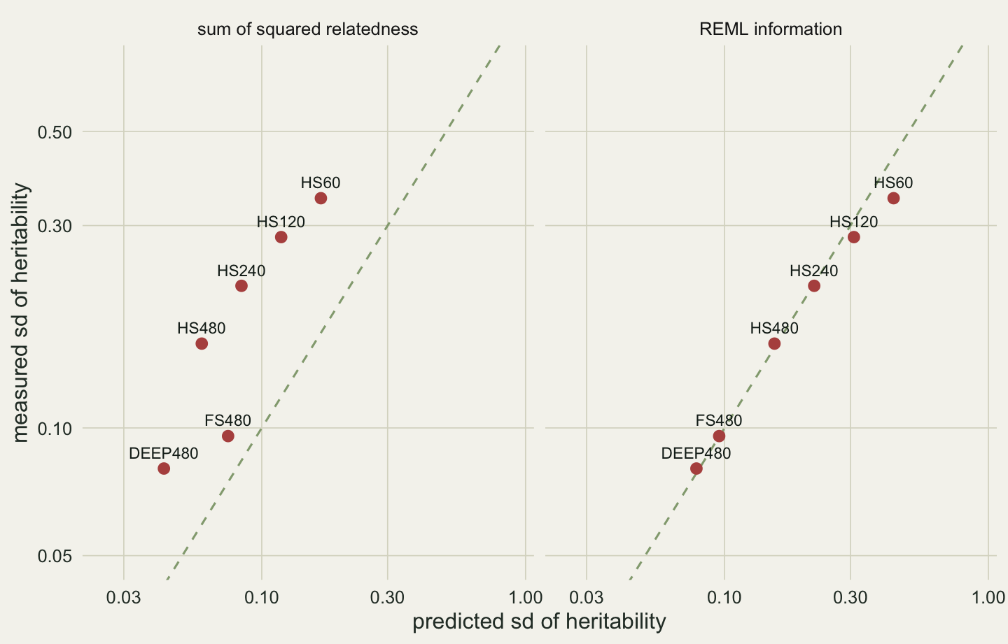
The figure above puts the six measured spreads against both predictions. Across sample sizes that differ by a factor of 8 and three family structures, the information calculation sits on the line of agreement except where the boundary bites, and the sum of squared relatedness sits off it everywhere, confidently and in one comparison backwards.
8.7 What the measurements say about design
n_equiv <- n_total * (sd_h2[["halfsib"]] / sd_h2[["deep"]])^2The number of phenotyped animals is a budget, not a measure of information. The same 480 animals gave standard deviations from 0.080 to 0.158 depending on how they were related, and no estimate at all when they were not related. To match the precision of the deep pedigree with the half-sib structure would take roughly 1,860 offspring instead of 480, by the square-root rule that the information calculation gives for designs clear of the boundary.
Several pieces of advice follow, and each rests on a measurement above. Close relatives are worth more than many distant ones whenever the heritability is expected to be above the crossover, which for most morphological traits it is; spreading the sample into large groups of weak relatives pays only for traits expected to be almost entirely environmental. Links that run across generations add contrasts that no single family structure provides, so a long-term study gains more from phenotyping the parents of the animals it measures, and from keeping parentage records unbroken across years, than from adding unrelated animals to any one cohort. And before the fieldwork, the pedigree the study expects to end with can be written down, A built from it, and asym_sd evaluated at a plausible heritability. It costs one eigen decomposition, and it says whether the design can answer the question at all. Where the answer comes back near the boundary, simulation replaces the formula. Real pedigrees of wild populations, of the kind Kruuk (2004) and Wilson and colleagues (2010) work with, are less complete than these simulated ones: a missing sire or an immigrant of unknown origin removes links, and every link removed costs precision.
The measurement has one limit that matters more than the others. Every design here was fitted with the model that generated it, so every design was precise about the right thing. The full-sib design owed its second place to the fact that each simulated animal had an environment of its own. A design that gains precision by packing relatives into families gains it through the comparisons that shared environments most easily counterfeit, and a design of full-sib families on its own cannot distinguish a resemblance inherited through genes from one acquired from a common mother. Kruuk and Hadfield (2007) set out how the two can be separated when the pedigree is rich enough. Chapter 9 adds a common-environment term to the animal model, measures what goes wrong when it is left out, and asks what a maternal effect does to the picture.
References
Henderson CR 1976. Biometrics 32(1):69-83 (10.2307/2529339)
Lynch M, Walsh B 1998. Genetics and Analysis of Quantitative Traits. Sinauer. ISBN 978-0878934812
Kruuk LEB 2004. Philosophical Transactions of the Royal Society B 359(1446):873-890 (10.1098/rstb.2003.1437)
Wilson AJ, Reale D, Clements MN, Morrissey MM, Postma E, Walling CA, Kruuk LEB, Nussey DH 2010. Journal of Animal Ecology 79(1):13-26 (10.1111/j.1365-2656.2009.01639.x)
Kruuk LEB, Hadfield JD 2007. Journal of Evolutionary Biology 20(5):1890-1903 (10.1111/j.1420-9101.2007.01377.x)