pcov <- function(x, y) mean(x * y) - mean(x) * mean(y)   # population moments, divisor n
V_A <- 4; V_E <- 6; mu <- 50
h2 <- V_A / (V_A + V_E); sd_P <- sqrt(V_A + V_E)

breed_counts <- function(a, W) {
  n <- length(a)
  if (sum(W) %% 2 == 1) {                                # gametes must pair up
    i <- sample(rep(seq_len(n), W), 1); W[i] <- W[i] - 1
  }
  slots <- sample(rep(seq_len(n), W))
  p1 <- slots[c(TRUE, FALSE)]; p2 <- slots[c(FALSE, TRUE)]
  ms <- rnorm(length(p1), 0, sqrt(V_A / 2))               # Mendelian sampling
  a_o <- (a[p1] + a[p2]) / 2 + ms
  list(W = W, p1 = p1, p2 = p2, ms = ms, a_o = a_o,
       z_o = mu + a_o + rnorm(length(p1), 0, sqrt(V_E)))
}

price <- function(x, x_off, g) {
  n <- length(x); w <- g$W / mean(g$W)
  tot <- tapply(c(x_off, x_off), factor(c(g$p1, g$p2), levels = seq_len(n)), sum)
  tot[is.na(tot)] <- 0
  delta <- ifelse(g$W > 0, tot / pmax(g$W, 1) - x, 0)    # offspring mean minus parent
  c(change = mean(x_off) - mean(x), selection = pcov(w, x),
    transmission = mean(w * delta))
}12 The Price equation and levels of selection
Chapter 11 closed Part III on a comparison of two variance ratios. Every prediction since Chapter 4 came from a model of how a mean changes, and each came with conditions under which it stopped saying anything useful. Part IV starts from the other end. Instead of a model of how a mean changes, it takes the change itself, after it has happened, and asks how it can be divided up. The division that answers the question is the Price equation (Price 1970). It holds in every population for every trait, whatever the genetics, and the predictions of Part II, together with the neutral drift of Chapter 11, reappear inside it as special cases, each obtained by saying what one of its two terms means in a particular setting.
This chapter derives it on a simulated population of parents and offspring and checks it to the precision of the arithmetic. It then recovers Robertson’s covariance form and the breeder’s equation from it, splits it a second time into selection between and within groups, and builds a population in which cooperators lose ground inside every group while becoming more common overall. The last section is about what the equation cannot do, which for an identity is a longer list than for a model.
12.1 Change in a mean, divided exactly
Label the parents \(i = 1, \dots, n\). Parent \(i\) has a trait value \(z_i\) and leaves \(W_i\) offspring, so its relative fitness is \(w_i = W_i / \bar W\). Its offspring have an average trait value \(z'_i\), and the difference \(\delta_i = z'_i - z_i\) is what happens to the trait on the way from parent to offspring. The mean of the offspring generation is the fitness-weighted mean of the \(z'_i\), and a line of algebra rearranges its difference from the parental mean into
\[ \Delta \bar z = \operatorname{cov}(w, z) + \operatorname{E}(w\,\delta). \]
The first term is the selection differential S of Chapter 1: the covariance between relative fitness and the trait among the parents. The second is transmission, the fitness-weighted average of the change between each parent and its own offspring. Nothing has been assumed about why fitness covaries with the trait or why offspring differ from their parents. Both terms are descriptions of what happened, and the equation says that together they account for the whole of the change.
A check needs a population with real parents and real offspring, not expected values. The engine below uses the genetic set-up of Chapter 4, a phenotype that is a breeding value plus an environmental deviation, and adds fitness as a count. Each parent contributes one gamete per offspring it produces; the gametes are shuffled and paired, so mating is random among the parents that breed, and each offspring inherits the average of its two parents’ breeding values plus a Mendelian sampling term. The function price() computes the two terms for any trait from the parents’ values, their offspring counts and the list of who is whose parent.
The first population has a fitness that rises with the phenotype on a log scale, with an expected family size of two.
set.seed(1201)
n <- 20000
b_fit <- 0.25                                            # log-fitness slope per SD of z
a <- rnorm(n, 0, sqrt(V_A)); z <- mu + a + rnorm(n, 0, sqrt(V_E))
W0 <- rpois(n, 2 * exp(b_fit * (z - mu) / sd_P - b_fit^2 / 2))
g <- breed_counts(a, W0)
pz <- price(z, g$z_o, g)
stopifnot(abs(pz["change"] - pz["selection"] - pz["transmission"]) < 1e-10)
n_off <- length(g$z_o)
barren <- mean(g$W == 0)
w <- g$W / mean(g$W)
gap_cov <- cov(w, z) - pcov(w, z)                        # sample covariance, divisor n - 1
The 20,000 parents leave 20,016 offspring, and 16 per cent of the parents leave none. The mean phenotype rises by 0.294. The selection term is 0.799 and the transmission term is -0.505, and their sum matches the observed change to the precision of the arithmetic, which is what the stopifnot() line checks. Parents with no offspring stay in the calculation: they have no \(\delta_i\), but their fitness of zero is part of the covariance, and dropping them would change both terms.
Exactness also depends on a detail of arithmetic. The covariance in the equation uses the divisor \(n\), the population covariance of the parents as they were, and R’s cov() divides by \(n - 1\). With the sample version the two sides disagree by \(4.00 \times 10^{-5}\), tiny against the terms themselves but enough to fail a check that should pass exactly, and an identity that only holds approximately is no longer being checked at all.
12.2 Robertson’s covariance and the breeder’s equation
The Price equation applies to any quantity that can be measured on parents and averaged over their offspring, and the breeding value is such a quantity. Run the same accounting with a in place of z. The offspring’s breeding value is the mean of its parents’ plus a Mendelian sampling term with mean zero, so the transmission term for a is the average Mendelian deviation of the offspring actually born, and it is unbiased in aggregate. A single parent’s offspring do differ from it, since half of each offspring’s breeding value comes from the mate, but each offspring is counted once for each parent and the two parents’ deviations from the midparent cancel, so what remains is the Mendelian term, with mean zero.
pa <- price(a, g$a_o, g)
stopifnot(abs(pa["change"] - pa["selection"] - pa["transmission"]) < 1e-10,
          abs(pa["transmission"] - mean(g$ms)) < 1e-10)
se_ms <- sd(g$ms) / sqrt(n_off)
S <- pz["selection"]
b_az <- pcov(a, z) / pcov(z, z)                          # regression of a on z in the parents
resid_cov <- pcov(w, a - b_az * z)
stopifnot(abs(pa["selection"] - (b_az * S + resid_cov)) < 1e-10)
se_resid <- sqrt(pcov(a - b_az * z, a - b_az * z)) * sd(w) / sqrt(n)
The mean breeding value rises by 0.319. Of that, 0.313 is the covariance between breeding value and relative fitness, and 0.005 is the mean Mendelian deviation, 0.5 standard errors from zero (standard error 0.010). So the Price equation for breeding values, with unbiased transmission, is Robertson’s (1966) form of Chapter 4, \(R = \operatorname{cov}(a, w)\), plus the noise of meiosis in one finite generation.
The breeder’s equation takes one more step. The covariance of fitness with breeding value can be split exactly, by regressing a on z among the parents, into \(b_{a|z}\,S\) and the covariance of fitness with the part of the breeding value the phenotype does not predict. The regression slope in this sample is 0.403, an estimate of h^2 = 0.40, and the leftover covariance is -0.008 with a standard error of about 0.008. When fitness depends on the phenotype and on nothing correlated with the breeding value beyond it, that leftover has an expectation of zero, and \(R = h^2 S\) is what remains. The breeder’s equation is therefore the Price equation with two claims added: transmission of breeding values is unbiased, and selection reaches the breeding value only through the phenotype, on which the breeding value has a linear regression, as it does when both are normal. The multivariate response of Chapter 5 is the same argument with vectors: the covariance of fitness with each trait’s breeding value, which that chapter compared with Lande’s (1979) \(\mathbf G \boldsymbol\beta\), is the selection term of the Price equation applied to each breeding value in turn.
The phenotype itself tells the complementary story. Its selection term is the whole differential S, but offspring inherit only the breeding values of their parents and draw fresh environments, so the transmission term for z should be close to \(-(1 - h^2)S\): the environmental part of the parents’ advantage is lost between generations. A single population is noisy, so the chunk below repeats the whole generation.
n_small <- 5000
one_rep <- function(n = n_small) {
  a <- rnorm(n, 0, sqrt(V_A)); z <- mu + a + rnorm(n, 0, sqrt(V_E))
  g <- breed_counts(a, rpois(n, 2 * exp(b_fit * (z - mu) / sd_P - b_fit^2 / 2)))
  pz <- price(z, g$z_o, g); pa <- price(a, g$a_o, g)
  c(trans_a = unname(pa["transmission"]),
    rob_gap = unname(pa["selection"] - h2 * pz["selection"]),
    trans_z_gap = unname(pz["transmission"] + (1 - h2) * pz["selection"]),
    S = unname(pz["selection"]))
}
set.seed(1202)
n_rep <- 200
reps <- t(replicate(n_rep, one_rep()))
rep_mean <- colMeans(reps); rep_se <- apply(reps, 2, sd) / sqrt(n_rep)
Over 200 replicate generations of 5,000 parents, the selection differential averages 0.793. The transmission term for breeding values averages 0.0001 (Monte Carlo standard error 0.0014), the gap between \(\operatorname{cov}(a, w)\) and \(h^2 S\) averages -0.0009 (standard error 0.0012), and the phenotypic transmission term differs from \(-(1-h^2)S\) by -0.0013 on average (standard error 0.0040). All three are zero within sampling error. Heritability, in this reading, is the share of the phenotypic selection term that survives transmission.
Drift, the process behind Chapter 11, has a place in the same accounting. In a finite population the covariance between fitness and breeding value is a sample quantity, and it is not zero in any one generation even when fitness has nothing to do with the trait. The chunk below gives every parent the same expected family size and records the change in the mean breeding value.
neutral_rep <- function(n = n_small) {
  a <- rnorm(n, 0, sqrt(V_A))
  g <- breed_counts(a, rpois(n, 2))                      # fitness unrelated to anything
  pa <- price(a, g$a_o, g)
  c(change = unname(pa["change"]), selection = unname(pa["selection"]),
    transmission = unname(pa["transmission"]))
}
set.seed(1206)
n_neutral <- 400
neu <- t(replicate(n_neutral, neutral_rep()))
drift_var <- apply(neu, 2, var)
drift_pred <- V_A / n_small                             # V_A / N for Poisson family sizes
drift_var_se <- drift_var["change"] * sqrt(2 / (n_neutral - 1))
drift_mean_se <- sqrt(drift_var["change"] / n_neutral)
Across 400 neutral generations the change in mean breeding value averages -0.0026 (standard error 0.0014), but its variance is 0.00077, with a standard error of about 0.00005, against 0.00080 expected from V_A divided by the number of parents, the amount by which the among-population variance of Chapter 11, twice \(F_{ST}\) times the ancestral V_A, grows in one generation when \(F_{ST}\) rises by one over twice the number of parents. The Price equation shows where that variance comes from: 0.00038 is the variance of the selection term, chance covariance between breeding value and family size, and 0.00037 is the variance of the transmission term, the Mendelian sampling of the offspring actually born. Drift is the two terms of the equation evaluated in a population too small for either to vanish.
12.3 The same accounting when selection runs through condition
Chapter 4 ended with a population in which a female’s condition set both her breeding date and her number of young, so that the phenotype was under apparent selection and did not evolve (Price, Kirkpatrick and Arnold 1988). The Price equation does not fail in that population; nothing can make an identity fail. What it does is show where the differential goes.
set.seed(1203)
cond <- rnorm(n)
a_c <- rnorm(n, 0, sqrt(V_A))
z_c <- mu + a_c + sqrt(V_E) * (0.7 * cond + sqrt(1 - 0.7^2) * rnorm(n))
g_c <- breed_counts(a_c, rpois(n, 2 * exp(0.4 * cond - 0.4^2 / 2)))
pz_c <- price(z_c, g_c$z_o, g_c); pa_c <- price(a_c, g_c$a_o, g_c)
stopifnot(abs(pz_c["change"] - sum(pz_c[-1])) < 1e-10,
          abs(pa_c["change"] - sum(pa_c[-1])) < 1e-10)
w_c <- g_c$W / mean(g_c$W)
se_cov_c <- sd(a_c) * sd(w_c) / sqrt(n)
The phenotypic selection term is 0.698, somewhat weaker than the 0.799 of the first population but of the same order, and the transmission term is -0.689, which takes back almost all of it: the mean phenotype moves by 0.010, and that movement is the Mendelian and environmental noise of one generation, which the breeding values show directly. Their selection term, \(\operatorname{cov}(a, w)\), is 0.016 with a standard error of about 0.012, and the mean breeding value changes by 0.014. Figure 12.1 sets the two populations side by side.
terms <- rbind(
  data.frame(pop = "fitness through the phenotype", trait = "phenotype z",
             term = names(pz), value = unname(pz)),
  data.frame(pop = "fitness through the phenotype", trait = "breeding value a",
             term = names(pa), value = unname(pa)),
  data.frame(pop = "fitness through condition", trait = "phenotype z",
             term = names(pz_c), value = unname(pz_c)),
  data.frame(pop = "fitness through condition", trait = "breeding value a",
             term = names(pa_c), value = unname(pa_c)))
terms$term <- factor(terms$term, levels = c("selection", "transmission", "change"),
                     labels = c("selection", "transmission", "net change"))
terms$pop <- factor(terms$pop, levels = unique(terms$pop))
terms$trait <- factor(terms$trait, levels = c("phenotype z", "breeding value a"))
ggplot(terms, aes(trait, value, fill = term)) +
  geom_hline(yintercept = 0, colour = te_body, linewidth = 0.3) +
  geom_col(position = position_dodge(width = 0.75), width = 0.7) +
  facet_wrap(~ pop) +
  scale_fill_manual(values = c(selection = te_forest, transmission = te_rust,
                               `net change` = te_gold), name = NULL) +
  labs(x = NULL, y = "contribution to the change in the mean") +
  theme_book()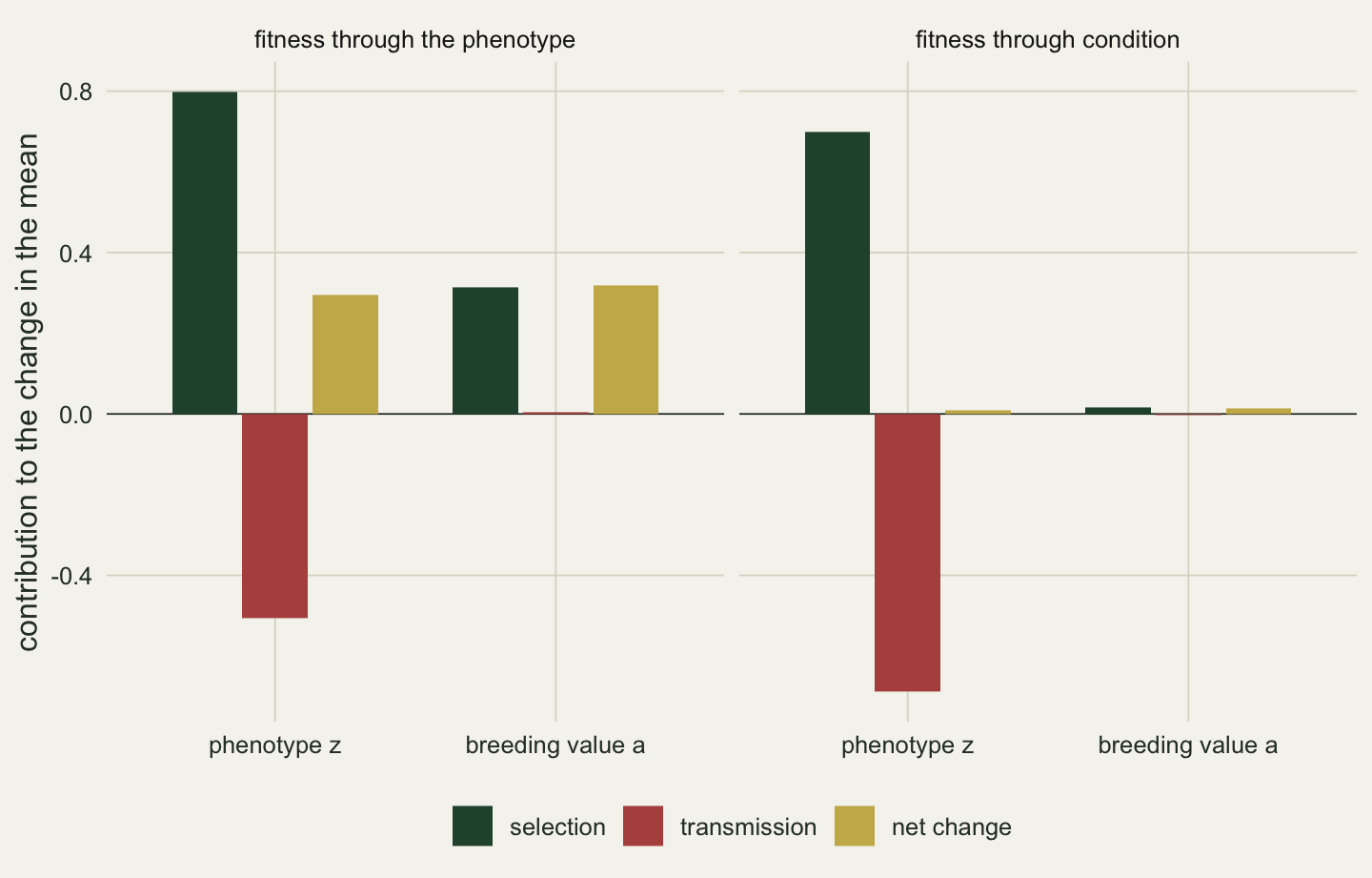
For the phenotype the two populations have selection terms of similar size and differ mainly in transmission. In the first, transmission removes the environmental share of the differential; in the second, the whole differential was environmental and transmission removes all of it. Robertson’s form is the Price equation written for the one trait whose transmission is known to be unbiased, and that is why it gets the second population right when the breeder’s equation does not.
12.4 Selection within and between groups
The selection term can itself be divided. If the parents live in groups of equal size, the law of total covariance splits \(\operatorname{cov}(W, z)\), here in absolute fitness, into the covariance, across groups, between a group’s mean fitness and its mean trait, and the average, over groups, of the covariance between fitness and trait inside each group. Price (1972) wrote the equation in this nested form, in which the within-group term is itself a Price equation for each group. Wilson (1975) built a theory of group selection on trait groups, the temporary groups within which individuals interact before dispersing, and the nested covariance is the natural way to keep its books.
The trait here is a behaviour. Individuals live in groups of m; a cooperator (\(z = 1\)) pays a cost c in fitness and produces a benefit b shared equally by the other members of its group, and a defector (\(z = 0\)) pays nothing. Offspring copy their parent’s type, so transmission is perfect and all of the change comes from selection. Fitness is the expected number of offspring, so the calculation is deterministic.
m <- 10; b <- 5; cost <- 1; w_base <- 2
k <- c(1, 3, 5, 7, 9)                                    # cooperators per group
grp <- rep(seq_along(k), each = m)
zc  <- unlist(lapply(k, function(kk) rep(c(1, 0), c(kk, m - kk))))
mates <- (k[grp] - zc) / (m - 1)                         # cooperator share among groupmates
wc  <- w_base - cost * zc + b * mates
x_g <- tapply(zc, grp, mean); w_g <- tapply(wc, grp, mean)
between <- pcov(w_g, x_g)
within  <- mean(sapply(split(seq_along(zc), grp), function(i) pcov(wc[i], zc[i])))
total   <- pcov(wc, zc)
x_after <- tapply(wc * zc, grp, sum) / tapply(wc, grp, sum)
p0 <- mean(zc); p1 <- sum(wc * zc) / sum(wc)
stopifnot(abs(total - between - within) < 1e-12,
          abs((p1 - p0) - total / mean(wc)) < 1e-12,
          abs(mean(w_g * (x_after - x_g)) - within) < 1e-12,   # nested form
          all(x_after < x_g), p1 > p0)
gap_coop <- cost + b / (m - 1)
There are 5 groups of 10, holding from 1 to 9 cooperators, with b = 5, c = 1 and a baseline fitness of 2. Inside every group a cooperator has lower fitness than a defector by 1.556, the cost plus the share of its own benefit that goes to the defector it is compared with, and that gap does not depend on how many cooperators the group holds. The within-group term is accordingly negative, -0.264. The between-group term is 0.320, because groups with more cooperators produce more offspring, and the total, 0.056, is positive. Divided by mean fitness it moves the cooperator frequency from 0.500 to 0.514, while the frequency inside each group falls. The stopifnot() line checks the split, the nested form and both directions of change.
simp <- rbind(
  data.frame(unit = paste("group", seq_along(k)), when = "before", x = unname(x_g)),
  data.frame(unit = paste("group", seq_along(k)), when = "after", x = unname(x_after)),
  data.frame(unit = "population", when = c("before", "after"), x = c(p0, p1)))
simp$when <- factor(simp$when, levels = c("before", "after"))
simp$level <- ifelse(simp$unit == "population", "whole population", "single group")
ggplot(simp, aes(when, x, group = unit, colour = level, linewidth = level)) +
  geom_line() +
  geom_point(size = 2.2) +
  scale_colour_manual(values = c(`single group` = te_rust, `whole population` = te_forest),
                      name = NULL) +
  scale_linewidth_manual(values = c(`single group` = 0.6, `whole population` = 1.4),
                         name = NULL) +
  scale_y_continuous(limits = c(0, 1)) +
  labs(x = NULL, y = "cooperator frequency") +
  theme_book()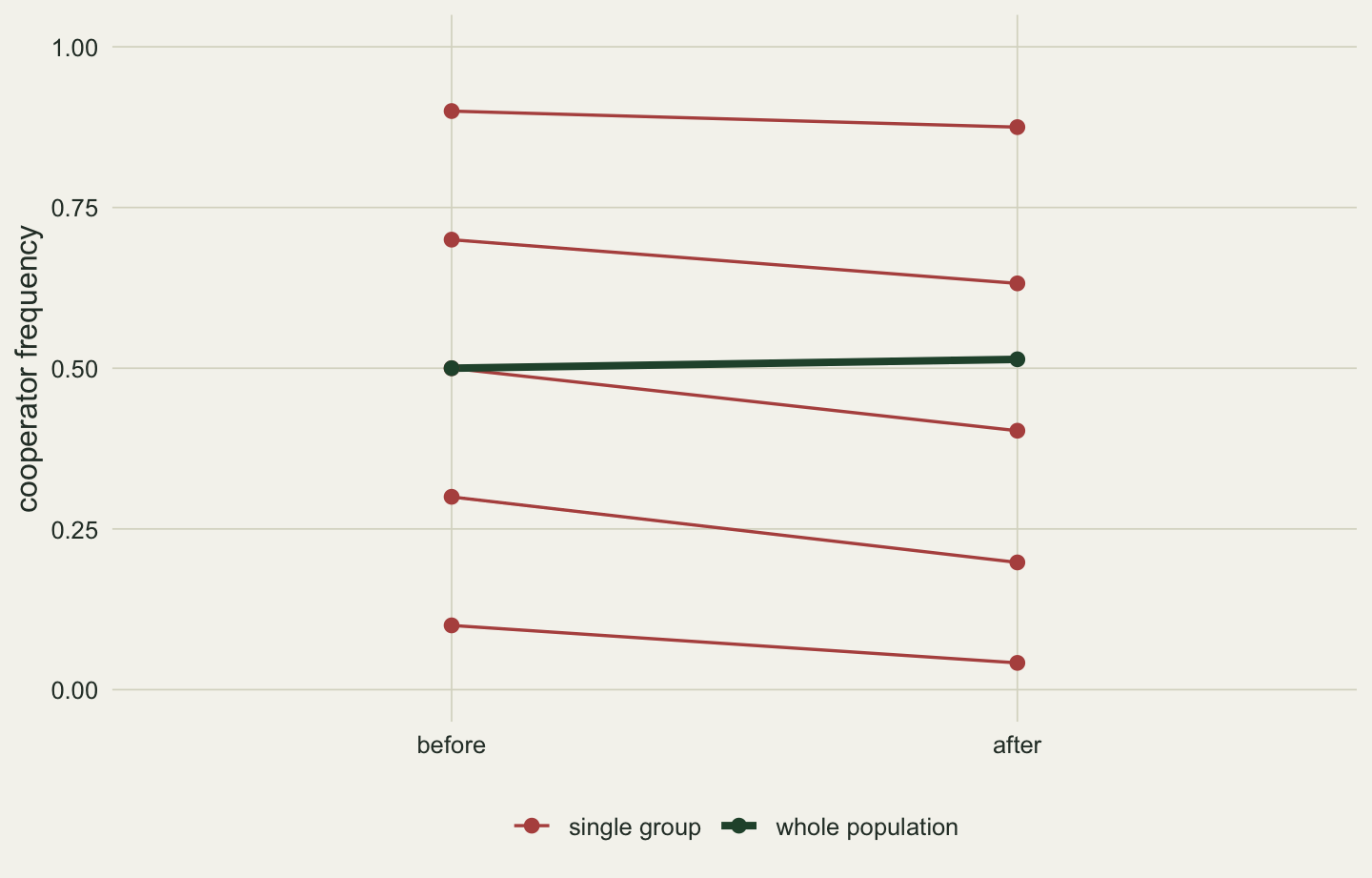
Figure 12.2 is Simpson’s paradox with a generation between the two panels of the table. Each group’s composition erodes, but the groups that erode from a higher starting point also contribute more of the next generation, and the shift of weight towards them outweighs the average loss of cooperators within groups.
12.5 The same change as a regression
The group accounting is one way to divide the selection term. Another way uses the structure of the fitness function itself. In this model an individual’s fitness is its baseline, minus c times its own trait, plus b times the cooperator share among its groupmates. Taking the covariance of each piece with the individual’s own trait gives, exactly,
\[ \operatorname{cov}(W, z) = \operatorname{var}(z)\,(r b - c), \]
where \(r\) is the slope of the regression of the groupmates’ mean trait on the individual’s own trait. Queller (1992) derived Hamilton’s rule by this route, splitting the selection covariance into a direct part and a part that passes through the traits of others.
r_mates <- pcov(mates, zc) / pcov(zc, zc)
F_grp   <- pcov(x_g, x_g) / (p0 * (1 - p0))                # share of variance between groups
n_grp <- 40; n_draw <- 2000                                # for the next section
stopifnot(abs(total - pcov(zc, zc) * (r_mates * b - cost)) < 1e-12,
          abs(r_mates - (m * F_grp - 1) / (m - 1)) < 1e-12)
In the five-group population \(r\) is 0.244, so \(rb\) = 1.222 exceeds c = 1 and the covariance is positive, as the group accounting found. The chunk also checks a second identity that ties \(r\) to the group structure: 32.0 per cent of the variance in the trait lies between groups, and \(r\) is that share, rescaled so that a group formed at random, with a between-group share of one in m, has an \(r\) of zero. The between-group share is the quantity Chapter 11 called Fst, here for a behavioural type instead of an allele. So the two divisions of one covariance are the same statement: between-group selection outweighs within-group selection exactly when \(rb > c\), and \(r\) measures how far group composition departs from random assortment.
That makes it possible to ask how groups have to form for cooperation to increase. The chunk below draws 2,000 populations of 40 groups of ten under three rules: individuals assorted at random from a population in which half are cooperators, and groups founded by five or by two individuals drawn at random, whose offspring fill the group.
r_from_x <- function(x) {                                  # x: cooperator fraction per group
  p <- mean(x); if (p == 0 || p == 1) return(NA)
  (m * pcov(x, x) / (p * (1 - p)) - 1) / (m - 1)
}
draw_x <- function(founders) {
  if (founders == 0) return(rbinom(n_grp, m, 0.5) / m)     # random assortment
  f_mean <- rbinom(n_grp, founders, 0.5) / founders
  rbinom(n_grp, m, f_mean) / m                             # members copy a random founder
}
set.seed(1204)
rules <- c(`random assortment` = 0, `five founders` = 5, `two founders` = 2)
r_draws <- lapply(rules, function(f) replicate(n_draw, r_from_x(draw_x(f))))
n_up    <- sapply(r_draws, function(r) sum(r * b > cost, na.rm = TRUE))
coop_up <- n_up / n_draw
r_med   <- sapply(r_draws, median, na.rm = TRUE)
r_theory_found <- 1 / rules[-1]                            # founder-descent expectation
rd <- data.frame(rule = factor(rep(names(rules), each = n_draw), levels = names(rules)),
r = unlist(r_draws))
ggplot(rd, aes(r)) +
geom_histogram(bins = 60, fill = te_sage, colour = te_paper, linewidth = 0.1) +
geom_vline(xintercept = cost / b, colour = te_rust, linetype = "dashed") +
facet_wrap(~ rule, ncol = 1, scales = "free_y") +
labs(x = "regression of groupmates' trait on own trait (r)", y = "populations") +
theme_book()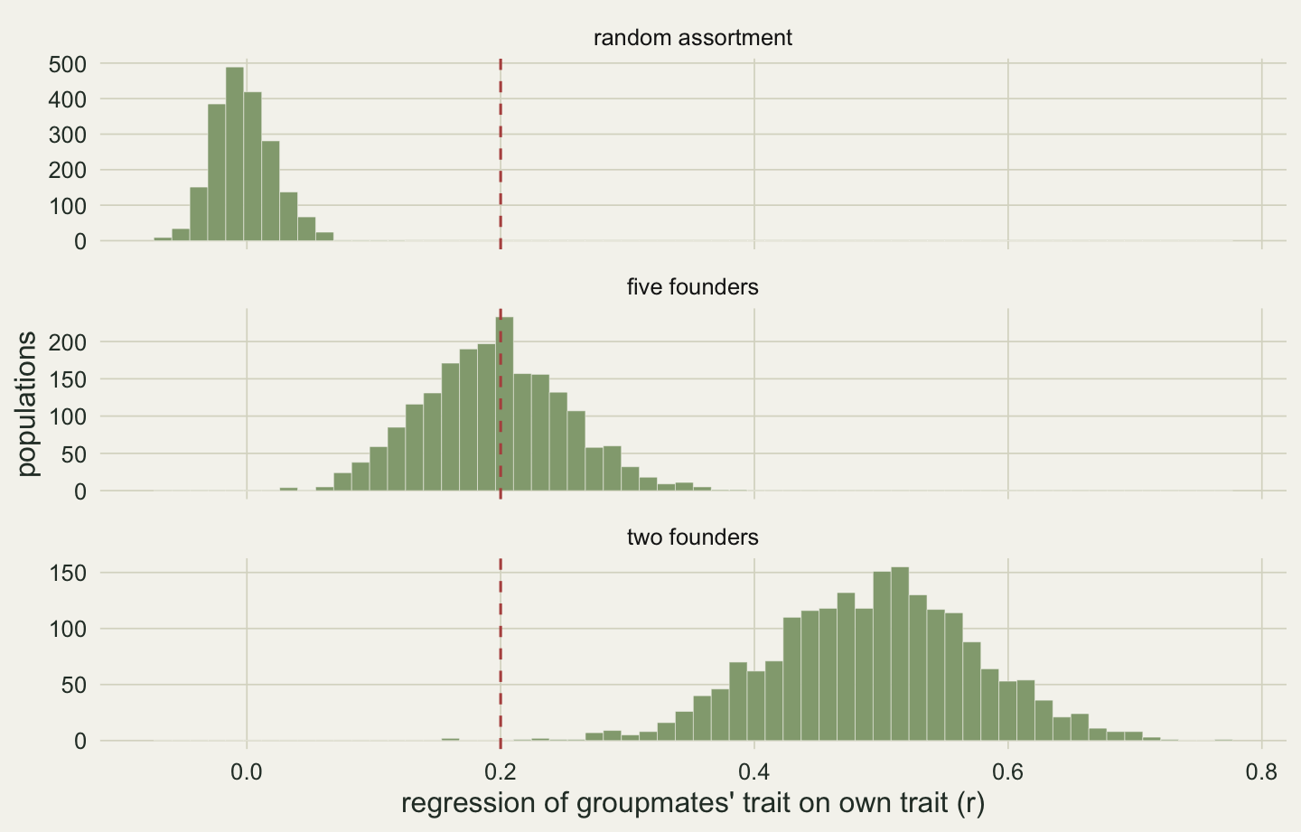
Under random assortment the median \(r\) is -0.005, and cooperators increase in 0 of the 2,000 draws: sampling noise alone does not supply enough variance between groups to beat the cost at this group size. The algebra says the same thing without simulation, since random groups have a between-group share of one in m on average and hence an expected \(r\) of zero, and \(rb > c\) can then hold only by chance. With five founders the median \(r\) is 0.194 and cooperators increase in 46 per cent of draws; with two founders it is 0.498 and they increase in 1998 of the 2,000 (Figure 12.3). In these founder groups each member copies one founder, so two groupmates are identical when they copy the same one and independent otherwise, and the expected \(r\) is the probability that they share a founder: 0.20 with five founders and 0.50 with two. Five founders put the expected \(r\) exactly on the threshold \(c/b\), which is why cooperation wins in a little under half of those populations and loses in the rest. Group selection strong enough to favour a costly trait came here only from groups of relatives.
12.6 What an identity can tell, and what it cannot
The Price equation holds for every population, and that is both its value and its limit. Its value is that it forces an account to be complete. A claim that a trait evolved by selection must be a claim about a covariance with fitness, and a claim that it did not evolve despite selection must be a claim about transmission. The condition example shows the discipline at work: the phenotypic account says, without any model, that the differential was real and that almost none of it was transmitted, which points directly at the covariance between fitness and breeding value as the quantity to estimate, as Morrissey and colleagues (2010) argued.
Its limit is that the terms are covariances, and a covariance is not a cause. In the condition example the phenotype has a selection term of the same order as in the population where it causes fitness, yet the phenotype does not affect fitness at all. The equation assigns the change correctly and says nothing about why fitness and trait covary. Worse for the multilevel reading, the division into levels is chosen by the analyst, and the change does not care which division is chosen.
set.seed(1205)
acc <- sample(grp)                                         # arbitrary accounting groups
x_acc <- tapply(zc, acc, mean); w_acc <- tapply(wc, acc, mean)
between_acc <- pcov(w_acc, x_acc)
within_acc  <- mean(sapply(split(seq_along(zc), acc), function(i) pcov(wc[i], zc[i])))
stopifnot(abs(between_acc + within_acc - total) < 1e-12)
Keep the same individuals and the same fitnesses, which were set by the real groups, but draw the accounting boundaries at random. The between-group term becomes 0.024 and the within-group term 0.032, and they still sum to the same total of 0.056. With the wrong boundaries, selection within groups appears to favour cooperators, because the accounting groups mix individuals whose fitness was set elsewhere. An identity cannot tell which boundaries are the biologically real ones; only knowledge of who interacts with whom can. The same holds for the choice between the group account and the regression account of the previous section: they are two divisions of one number, and a dispute between them is a dispute about bookkeeping unless it names a measurement that would come out differently. Frank (1998) sets out this equivalence between the group and the kin accounts at length.
The equation also looks back rather than forward. Every term is computed from a generation that has already happened, and projecting the next generation requires knowing how the covariance and the transmission term will change, which means a model again. Here the groups were fixed for one round; whether cooperation keeps increasing depends on how offspring disperse and new groups form, and the assortment simulation shows that a single round of random regrouping would remove the excess variance between groups that the between-group term feeds on.
12.7 From groups to relatives
The regression slope \(r\) did all the work in the second half of this chapter. It decided the sign of the change, it was a rescaled share of variance between groups, and it was large only when groupmates shared founders. Chapter 13 takes that slope out of the group setting. It treats relatedness as a regression coefficient of a partner’s trait on an actor’s, compares it with the pedigree coefficients of the relationship matrix A in Chapter 7, and reads Hamilton’s rule, \(rb > c\), as a statement about regression coefficients that holds exactly in the population where they are measured.
References
Price GR 1970. Nature 227(5257):520-521 (10.1038/227520a0)
Price GR 1972. Annals of Human Genetics 35(4):485-490 (10.1111/j.1469-1809.1957.tb01874.x)
Robertson A 1966. Animal Production 8(1):95-108 (10.1017/S0003356100037752)
Lande R 1979. Evolution 33(1):402-416 (10.1111/j.1558-5646.1979.tb04694.x)
Price T, Kirkpatrick M, Arnold SJ 1988. Science 240(4853):798-799 (10.1126/science.3363360)
Wilson DS 1975. Proceedings of the National Academy of Sciences 72(1):143-146 (10.1073/pnas.72.1.143)
Queller DC 1992. Evolution 46(2):376-380 (10.1111/j.1558-5646.1992.tb02045.x)
Morrissey MB, Kruuk LEB, Wilson AJ 2010. Journal of Evolutionary Biology 23(11):2277-2288 (10.1111/j.1420-9101.2010.02084.x)
Frank SA 1998. Foundations of Social Evolution. Princeton University Press. ISBN 978-0691059341