p_anc  <- 0.5
n_loci <- 100
va_anc <- 1                       # ancestral additive variance
h2_pop <- 0.3                     # heritability in the common garden
ve_com <- va_anc * (1 - h2_pop) / h2_pop

draw_pops <- function(n_pop, fst, spread = 1) {
  sh1 <- p_anc * (1 - fst) / fst
  sh2 <- (1 - p_anc) * (1 - fst) / fst
  p_mat <- matrix(rbeta(n_pop * n_loci, sh1, sh2), nrow = n_pop)
  a_eff <- sqrt(va_anc / (2 * n_loci * p_anc * (1 - p_anc)))
  mu_anc <- 2 * a_eff * n_loci * p_anc
  list(mu = mu_anc + spread * (2 * a_eff * rowSums(p_mat) - mu_anc),
       va = 2 * a_eff^2 * rowSums(p_mat * (1 - p_mat)))
}

# the algebra: Qst from the expected components equals Fst whatever L, a and p are
qst_expected <- function(fst, L, a, p) {
  vb <- 4 * L * a^2 * fst * p * (1 - p)
  va <- 2 * L * a^2 * p * (1 - p) * (1 - fst)
  vb / (vb + 2 * va)
}
chk <- expand.grid(fst = c(0.02, 0.1, 0.3), L = c(1, 10, 500),
                   a = c(0.1, 2), p = c(0.1, 0.5))
stopifnot(max(abs(with(chk, qst_expected(fst, L, a, p)) - chk$fst)) < 1e-12)

fst_mark  <- 0.10
alpha_lev <- 0.05
n_pop_cal <- 40
n_cal     <- 3000
set.seed(1101)
cal <- t(vapply(seq_len(n_cal), function(i) {
  pp <- draw_pops(n_pop_cal, fst_mark)
  c(vb = var(pp$mu), va = mean(pp$va))
}, numeric(2)))
vb_cal  <- mean(cal[, "vb"]); vb_pred <- 2 * fst_mark * va_anc
va_cal  <- mean(cal[, "va"]); va_pred <- (1 - fst_mark) * va_anc
vb_se   <- sd(cal[, "vb"]) / sqrt(n_cal)
va_se   <- sd(cal[, "va"]) / sqrt(n_cal)
qst_cal <- vb_cal / (vb_cal + 2 * va_cal)
stopifnot(abs(vb_cal - vb_pred) < 4 * vb_se, abs(va_cal - va_pred) < 4 * va_se)11 Qst against Fst
Chapter 10 finished the audit of the animal model, and every variance component in Part III so far has belonged to a single population: the additive variance of one bird population, estimated from one pedigree and checked against the ways that particular fit can mislead. Many of the questions ecologists bring to quantitative genetics are about several populations at once. Two populations of a fish differ in body depth. Did selection push them apart, or did they drift apart, as neutral alleles do, because each was small and isolated? The standard answer compares two numbers. Fst, measured at neutral markers, is the share of the genetic variation at those loci that lies among populations rather than within them. Qst is the same share computed for the additive genetic variance of a trait. If a trait is more differentiated than the markers, the reasoning goes, something other than drift has been at work.
This chapter takes that comparison apart in the way the rest of the book has treated its estimators. It derives the neutral expectation, simulates the distribution of Qst that drift alone produces, measures how often a neutral trait beats Fst, and ends with what a test that deserves the name has to do. The running example is a common-garden study: several populations reared together, so that whatever difference remains between them in body depth is genetic, and a breeding design within each population so that the additive variance can be estimated. The markers return a moderate Fst, the value most simulations below are built around.
11.1 The neutral expectation
Take a trait built from \(L\) unlinked additive loci of equal effect \(\alpha\), so that a genotype carrying zero, one or two copies of the plus allele at a locus contributes nothing, \(\alpha\) or \(2\alpha\). An ancestral population sits at frequency \(p\) at every locus, and descendant populations drift apart independently. Under the usual model of drift the frequency in a descendant population varies around \(p\) with variance \(F_{ST}\,p(1-p)\), and the beta distribution with that mean and variance is the standard way to draw it.
The population mean at one locus is \(2\alpha p_j\), so its variance across populations is \(4\alpha^2F_{ST}\,p(1-p)\), and summing over loci gives the among-population variance of the mean breeding value, \(V_B = 4L\alpha^2F_{ST}\,p(1-p)\). Within a population the additive variance at one locus is \(2\alpha^2p_j(1-p_j)\), whose expectation over the drift process is \(2\alpha^2p(1-p)(1-F_{ST})\), so \(V_A = 2L\alpha^2p(1-p)(1-F_{ST})\). Qst for an additive trait is defined as
\[ Q_{ST} = \frac{V_B}{V_B + 2V_A}, \]
with the factor of two on the within-population term because the variance of a population mean under drift is twice \(F_{ST}\) times the ancestral additive variance, while the within-population term carries no such doubling. Substituting, every factor of \(L\), \(\alpha\) and \(p(1-p)\) cancels and \(Q_{ST} = F_{ST}\) exactly. Lande (1992) set out the neutral theory of quantitative divergence among populations in this form, and Spitze (1993) was among the first to use the equality as a null hypothesis with real data, on Daphnia.
The chunk checks the cancellation on a grid of 36 combinations of \(F_{ST}\), \(L\), \(\alpha\) and \(p\), where the two agree to the precision of the arithmetic, and then checks the generator that the rest of the chapter uses. The allelic effect is scaled so that the ancestral additive variance is 1.00. Over 3,000 replicate sets of 40 populations drifted to an Fst of 0.10, the among-population variance averages 0.201 against a predicted 0.200 (Monte Carlo standard error 0.001), the within-population additive variance averages 0.900 against 0.900, and the ratio of the averages is 0.100.
That last number is a ratio of expectations, which is exactly what the theorem is about. No study observes it. A study has one realisation of drift in a handful of populations, and a breeding design that estimates both variance components with error. The expected value of the ratio of two noisy estimates is not the ratio of their expectations, and the whole of the rest of the chapter lives in the gap between the two.
11.2 Estimating Qst in a common garden
The breeding design is the paternal half-sib design of Chapter 8 in its simplest balanced form. Within each population, each sire is mated to several dams and one offspring per dam is measured, so the offspring of a sire share half their sire’s breeding value and nothing else: no dam, no nest and none of the maternal environment that Chapter 9 showed can masquerade as additive resemblance. The variance among sires is then a quarter of V_A. With \(f\) sires per population and \(n\) offspring per sire, a nested analysis of variance gives three mean squares whose expectations are
\[ E[MS_E] = \sigma^2_E, \qquad E[MS_S] = \sigma^2_E + n\sigma^2_S, \qquad E[MS_P] = \sigma^2_E + n\sigma^2_S + fn\sigma^2_P , \]
and solving from the bottom up gives \(\hat V_A = 4\hat\sigma^2_S\) and \(\hat V_B = \hat\sigma^2_P = (MS_P - MS_S)/fn\). There is a shortcut that needs no analysis of variance at all: take the variance of the observed population means and call it \(V_B\). That variance is \(MS_P/fn\), and its expectation is \(\sigma^2_P + \sigma^2_S/f + \sigma^2_E/fn\): the among-population component plus the sampling variance of a mean. The two estimates differ by \(MS_S/fn\) in every data set, and since a mean square cannot be negative the shortcut can never return a smaller Qst than the nested analysis.
qst_ratio <- function(vb, va) {
  vb <- max(vb, 0); va <- max(va, 0)
  if (vb <= 0) return(0)            # no among-population variance
  if (va <= 0) return(1)            # among-population variance but no additive variance
  vb / (vb + 2 * va)
}
sim_garden <- function(n_pop, n_sire, n_off, fst, spread = 1) {
  pops <- draw_pops(n_pop, fst, spread)
  y <- array(0, dim = c(n_off, n_sire, n_pop))
  for (j in seq_len(n_pop)) {
    sire <- rnorm(n_sire, 0, sqrt(pops$va[j] / 4))
    y[, , j] <- rep(pops$mu[j] + sire, each = n_off) +
      rnorm(n_off * n_sire, 0, sqrt(0.75 * pops$va[j] + ve_com))
  }
  y
}
nested_qst <- function(y) {
  n_off <- dim(y)[1]; n_sire <- dim(y)[2]; n_pop <- dim(y)[3]
  fam_mean <- colMeans(y)
  pop_mean <- colMeans(fam_mean)
  ms_pop  <- n_sire * n_off * sum((pop_mean - mean(pop_mean))^2) / (n_pop - 1)
  ms_sire <- n_off * sum((fam_mean - rep(pop_mean, each = n_sire))^2) /
    (n_pop * (n_sire - 1))
  ms_err  <- sum((y - rep(as.vector(fam_mean), each = n_off))^2) /
    (n_pop * n_sire * (n_off - 1))
  v_sire  <- (ms_sire - ms_err) / n_off
  v_among <- (ms_pop - ms_sire) / (n_sire * n_off)
  v_naive <- ms_pop / (n_sire * n_off)
  c(qst = qst_ratio(v_among, 4 * v_sire), qst_naive = qst_ratio(v_naive, 4 * v_sire),
    v_among = v_among, v_naive = v_naive, ms_sire = ms_sire)
}

n_pop0 <- 6; n_sire0 <- 25; n_off0 <- 8
set.seed(1102)
garden <- sim_garden(n_pop0, n_sire0, n_off0, fst_mark)
one    <- nested_qst(garden)
n_fish <- length(garden)
d_one  <- data.frame(y = as.vector(garden),
                     pop  = factor(rep(seq_len(n_pop0), each = n_sire0 * n_off0)),
                     sire = factor(rep(seq_len(n_pop0 * n_sire0), each = n_off0)))
aov_tab <- summary(aov(y ~ pop + pop:sire, data = d_one))[[1]]
stopifnot(abs(aov_tab[1, "Mean Sq"] / (n_sire0 * n_off0) - one[["v_naive"]]) < 1e-8,
          abs(aov_tab[2, "Mean Sq"] - one[["ms_sire"]]) < 1e-8,
          abs(one[["v_naive"]] - one[["v_among"]] -
                one[["ms_sire"]] / (n_sire0 * n_off0)) < 1e-10)
One neutral garden, with 6 populations, 25 sires per population and 8 offspring per sire, makes 1,200 fish. The hand-written mean squares agree with those of aov() to the precision of the arithmetic, and so does the identity between the two estimators. This particular data set gives a nested Qst of 0.023 and a shortcut Qst of 0.036, both below the marker Fst of 0.10, so this study would find no divergence. A different seed puts the estimates on the other side of Fst just as easily. How often each side comes up is the operating characteristic of the rule “Qst above Fst means selection”, and it is the measurement this chapter is built around.
The shortcut’s bias is fixed by the design before any fish is measured, so it can be predicted and then checked. The sweep below holds the number of populations fixed and changes the number of sires and offspring.
replicate_qst <- function(n_pop, n_sire, n_off, fst, n_rep, spread = 1) {
  t(vapply(seq_len(n_rep),
           function(i) nested_qst(sim_garden(n_pop, n_sire, n_off, fst, spread)),
           numeric(5)))
}
mc_se <- function(p, n) sqrt(p * (1 - p) / n)
design_grid <- list(c(10, 4), c(15, 6), c(25, 8), c(40, 8), c(60, 10))
n_pop_des <- 8
n_rep_des <- 2000
sw_true <- (1 - fst_mark) * va_anc / 4
se_true <- 0.75 * (1 - fst_mark) * va_anc + ve_com
set.seed(1103)
des <- do.call(rbind, lapply(design_grid, function(dz) {
  r <- replicate_qst(n_pop_des, dz[1], dz[2], fst_mark, n_rep_des)
  data.frame(sires = dz[1], off = dz[2], per_pop = dz[1] * dz[2],
             bias_obs  = mean(r[, "v_naive"] - r[, "v_among"]),
             bias_pred = sw_true / dz[1] + se_true / (dz[1] * dz[2]),
             qst = mean(r[, "qst"]), qst_naive = mean(r[, "qst_naive"]),
             fpr = mean(r[, "qst"] > fst_mark),
             fpr_naive = mean(r[, "qst_naive"] > fst_mark),
             zero_frac = mean(r[, "qst"] <= 0), one_frac = mean(r[, "qst"] >= 1))
}))
bias_rel <- max(abs(des$bias_obs / des$bias_pred - 1))
Across the 5 designs, each with 8 populations and from 40 to 600 offspring per population, the observed inflation of the among-population variance matches the predicted \(\sigma^2_S/f + \sigma^2_E/fn\) to within 0.4 per cent. That is a check on the code rather than a result. At the smallest design the inflation is 0.098, which is 49 per cent of the true among-population component of 0.200; at the largest it is 0.009.
des_long <- rbind(
  data.frame(per_pop = des$per_pop, estimator = "nested ANOVA",
             panel = "mean estimated Qst", value = des$qst),
  data.frame(per_pop = des$per_pop, estimator = "spread of population means",
             panel = "mean estimated Qst", value = des$qst_naive),
  data.frame(per_pop = des$per_pop, estimator = "nested ANOVA",
             panel = "P(estimated Qst > Fst)", value = des$fpr),
  data.frame(per_pop = des$per_pop, estimator = "spread of population means",
             panel = "P(estimated Qst > Fst)", value = des$fpr_naive))
des_ref <- data.frame(panel = c("mean estimated Qst", "P(estimated Qst > Fst)"),
                      y = c(fst_mark, alpha_lev))
panel_lev <- c("mean estimated Qst", "P(estimated Qst > Fst)")
des_long$panel <- factor(des_long$panel, panel_lev)
des_ref$panel  <- factor(des_ref$panel, panel_lev)
ggplot(des_long, aes(per_pop, value, colour = estimator)) +
  geom_hline(data = des_ref, aes(yintercept = y), colour = te_ink, linetype = "dashed") +
  geom_line(linewidth = 0.9) + geom_point(size = 2.2) +
  facet_wrap(~ panel, scales = "free_y") +
  expand_limits(y = 0) +
  scale_x_log10(breaks = des$per_pop) +
  scale_colour_manual(values = c(`nested ANOVA` = te_forest,
                                 `spread of population means` = te_rust), name = NULL) +
  labs(x = "offspring per population (log scale)", y = NULL) +
  theme_book()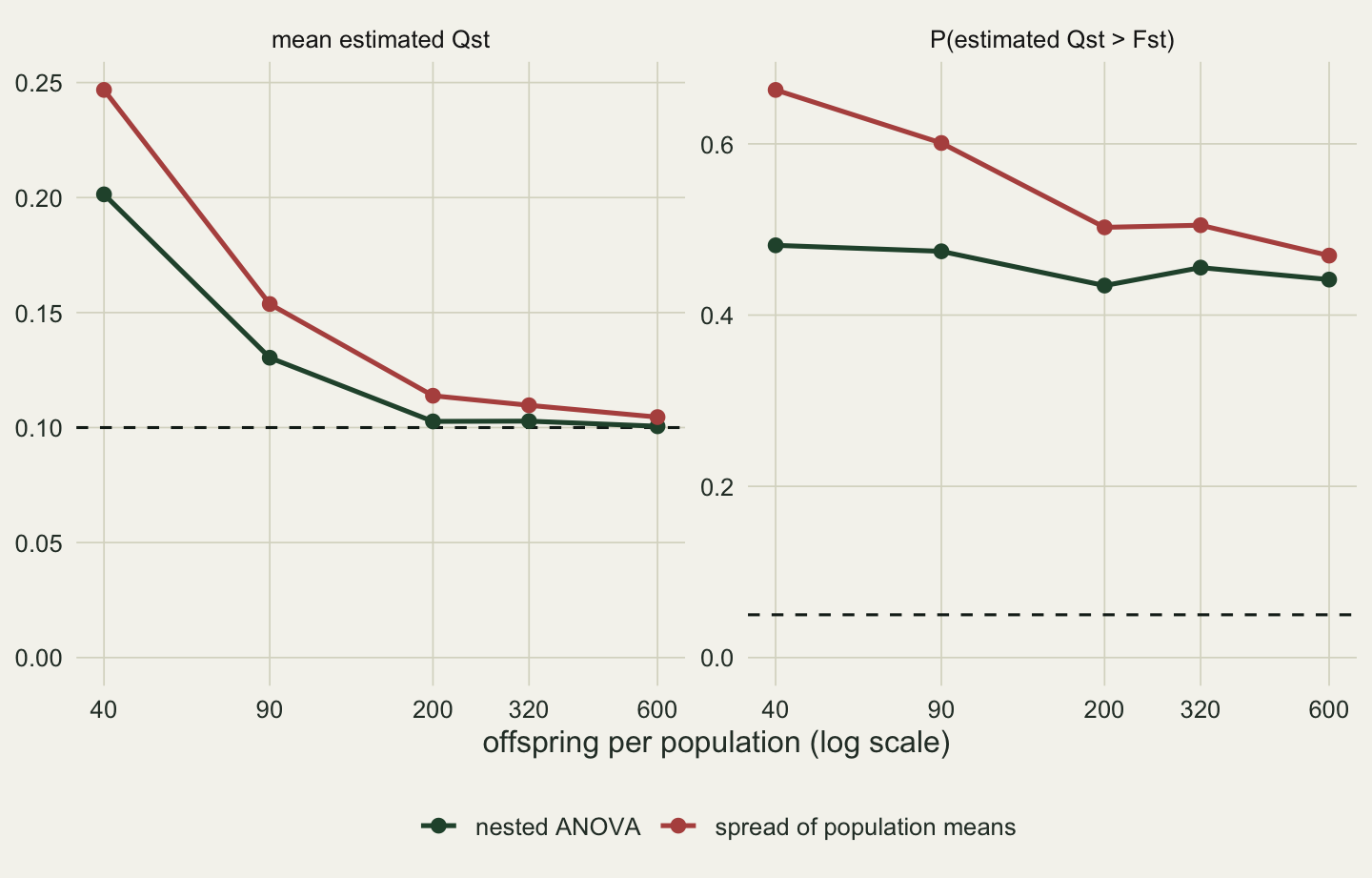
The left panel is the familiar story of a biased estimator: the shortcut sits above the truth by an amount that shrinks as the design grows, and the nested estimator, less biased, is still above the truth at small designs, largely because a replicate whose estimated V_A falls to zero is recorded as a Qst of one. The right panel is the story of this chapter. At the smallest design, removing the design bias lowers the rate at which the rule calls selection on neutral data from 66 to 48 per cent. After that, enlarging the design barely moves the nested rate, which is still 44 per cent at the largest design, where the shortcut has come down to 47 per cent. A bigger breeding design buys a better estimate of each variance component and does very little for the decision.
11.3 The drift null of Qst
The number of populations is the sample size of the among-population component, whatever the number of fish. The next simulation crosses a range of numbers of populations with a range of values of Fst at the intermediate design of 25 sires and 8 offspring, and records the whole distribution of the nested estimate under drift.
d_vec   <- c(3, 5, 8, 16, 32)
fst_vec <- c(0.02, 0.05, 0.10, 0.20)
k_big   <- 2.5                    # a "large" excess: Qst above 2.5 times Fst
n_rep   <- 4000
n_boot  <- 200
set.seed(1104)
null_raw <- list(); grid_rows <- list()
for (ff in fst_vec) for (dd in d_vec) {
  r <- replicate_qst(dd, n_sire0, n_off0, ff, n_rep)
  if (ff == fst_mark) null_raw[[as.character(dd)]] <- r[, "qst"]
  boot <- replicate(n_boot, quantile(sample(r[, "qst"], n_rep, TRUE), 1 - alpha_lev))
  grid_rows[[length(grid_rows) + 1]] <- data.frame(
    fst = ff, n_pop = dd, mean_qst = mean(r[, "qst"]), med_qst = median(r[, "qst"]),
    fpr = mean(r[, "qst"] > ff), fpr_naive = mean(r[, "qst_naive"] > ff),
    fpr_big = mean(r[, "qst"] > k_big * ff),
    q_crit = unname(quantile(r[, "qst"], 1 - alpha_lev)), q_crit_se = sd(boot))
}
grid_df <- do.call(rbind, grid_rows)
grid_df$mult <- grid_df$q_crit / grid_df$fst
grid_df$mult_se <- grid_df$q_crit_se / grid_df$fst
main <- grid_df[grid_df$fst == fst_mark, ]
se_max <- mc_se(0.5, n_rep)
stopifnot(all(main$med_qst < fst_mark), all(main$mean_qst > fst_mark))
ecdf_df <- do.call(rbind, lapply(names(null_raw), function(k)
data.frame(qst = null_raw[[k]], pops = factor(k, as.character(d_vec)))))
ggplot(ecdf_df, aes(qst, colour = pops)) +
geom_vline(xintercept = fst_mark, colour = te_ink, linetype = "dashed") +
stat_ecdf(linewidth = 0.8, pad = FALSE) +
coord_cartesian(xlim = c(0, 0.5)) +
scale_colour_manual(values = c(te_rust, te_gold, te_sage, te_forest, te_ink),
name = "populations") +
labs(x = "estimated Qst under drift alone", y = "cumulative probability") +
theme_book()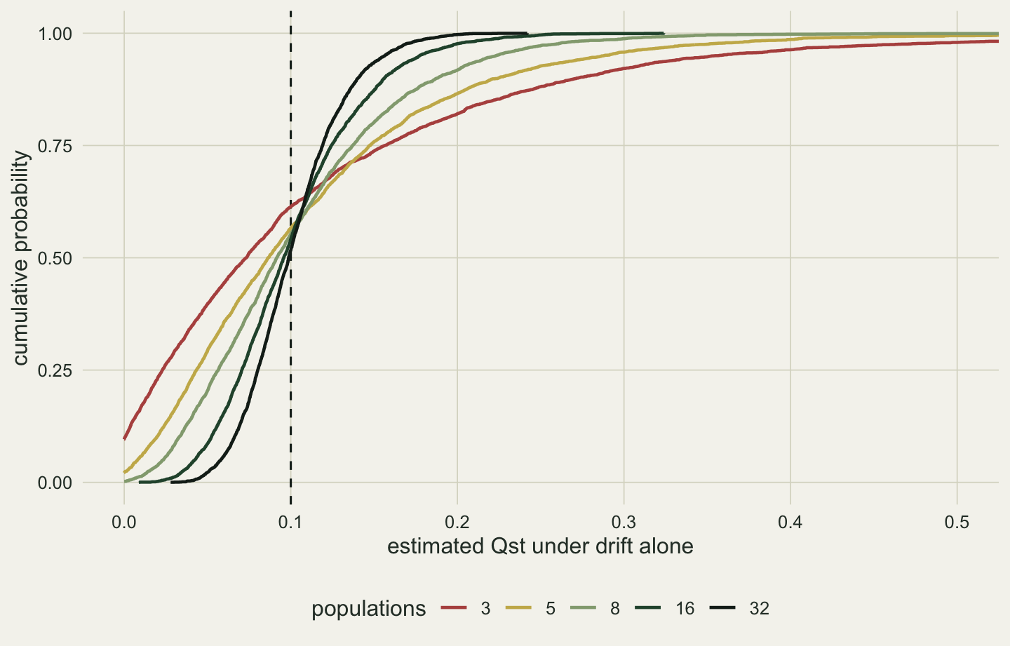
Two things are visible at once. The null is wide when populations are few: at 3 populations, 10 per cent of neutral data sets return a Qst of exactly zero and one in twenty returns more than 0.355, while at 32 populations the whole distribution is compressed around Fst. And the null is skewed. At 3 populations the median neutral estimate is 0.073 and the mean is 0.113, on either side of the Fst of 0.10 that the theorem points to. The mean lies a little above Fst at every number of populations, from 0.101 to 0.113, and the median lies below it at every one.
Because the median lies below Fst, a neutral estimate exceeds Fst somewhat less than half the time. The rate is 0.386 at 3 populations and 0.484 at 32, each with a Monte Carlo standard error of at most 0.008. Skew makes the rule look slightly better than a coin toss and no better than that. Across all 20 combinations of Fst and number of populations the lowest false-positive rate is 0.386, 7.72 times the nominal 0.05 of a test at the usual level.
11.4 Why a point comparison is not a test
A test is a rule with a known probability of rejecting a true null. “Qst above Fst” has a probability of rejecting a true null that is fixed by the geometry of the null distribution, not by the analyst, and the geometry puts it near one half. Stated this way it is plain that no amount of data can repair it: more populations narrow the null around Fst, but the point estimate still falls on each side of it roughly half the time, so the rule converges on a coin toss rather than on a test.
rule_lab <- c("Qst > Fst, nested ANOVA", "Qst > Fst, spread of means",
              "Qst > 2.5 Fst, nested ANOVA")
rate_df <- data.frame(n_pop = rep(main$n_pop, 3),
                      rate = c(main$fpr, main$fpr_naive, main$fpr_big),
                      rule = factor(rep(rule_lab, each = nrow(main)), rule_lab))
rate_df$se <- mc_se(rate_df$rate, n_rep)
ggplot(rate_df, aes(n_pop, rate, colour = rule)) +
  geom_hline(yintercept = alpha_lev, colour = te_ink, linetype = "dashed") +
  geom_errorbar(aes(ymin = rate - 2 * se, ymax = rate + 2 * se),
                width = 0.06, linewidth = 0.4) +
  geom_line(linewidth = 0.9) + geom_point(size = 2.2) +
  scale_x_log10(breaks = d_vec) +
  scale_colour_manual(values = setNames(c(te_forest, te_rust, te_gold), rule_lab),
                      name = NULL) +
  labs(x = "populations (log scale)", y = "false-positive rate under drift") +
  theme_book() + theme(legend.direction = "vertical")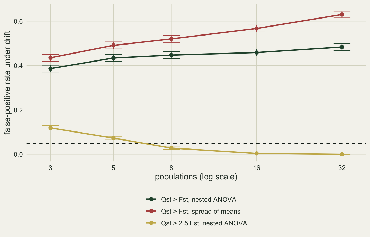
The green line is the rule applied to the nested estimate, and it climbs towards one half from below as the estimate concentrates on Fst. The red line is the same rule applied to the spread of population means, and it goes straight through one half: from 44 per cent of neutral data sets at 3 populations to 63 per cent at 32. Adding populations shrinks the noise around the shortcut’s centre, but the bias in that centre depends only on the breeding design, so the estimate converges on the wrong value and, with enough populations, the rule would fire on every neutral data set. The effect is larger when differentiation is weak, because the sampling variance of a mean is then a larger share of a small among-population component. At an Fst of 0.02 and 32 populations the shortcut calls selection on 95 per cent of neutral data sets.
The gold line is the rule most readers would reach for next: demand a clear excess, Qst above 2.50 times Fst, before calling selection. It is conservative with many populations and not with few. At 3 populations it fires on 11.9 per cent of neutral data sets, above the nominal level, and it only drops below 5 per cent somewhere between 5 and 8 populations. A fixed multiple is a critical value chosen without looking at the null it is meant to cut, and it is right, if at all, for one combination of design, Fst and number of populations.
Part of that upper tail is drift itself and part is estimation. If the population means and the within-population variance were known without error, the realised among-population variance under drift would be a scaled chi-squared variable on one fewer degrees of freedom than there are populations, and the probability of a Qst above 2.50 times Fst could be written down.
mult_big   <- (1 - fst_mark) * k_big / (1 - k_big * fst_mark)
drift_only <- pchisq(mult_big * (d_vec - 1), d_vec - 1, lower.tail = FALSE)
tail_ratio <- main$fpr_big / drift_only
With perfect measurement that probability would be 0.050 at 3 populations and 0.004 at 8. The simulated rates, 0.119 and 0.028, are 2.39 and 7.43 times as large. Drift alone produces a wide null when populations are few; the breeding design widens it further, and the share of the tail owed to estimation grows as the drift part shrinks. Whitlock (2008) made the general version of this argument: the neutral distribution of Qst is wide and skewed enough that one estimate set against one number carries very little evidence.
11.5 What a proper test needs
The repair that Whitlock and Guillaume (2009) proposed follows directly from the diagnosis. The critical value has to come from the neutral distribution of the Qst estimate for the design, the number of populations and the Fst actually in hand, and the natural way to get that distribution is to simulate it, as this chapter has. Their full version also carries the sampling error of Fst, which the simulations here treat as known. Expressed as a multiple of Fst, the critical value of a one-sided 5 per cent test is the 95th percentile of the null divided by Fst.
grid_df$fst_lab <- factor(sprintf("Fst = %.2f", grid_df$fst))
ggplot(grid_df, aes(n_pop, mult, colour = fst_lab)) +
  geom_hline(yintercept = 1, colour = te_ink, linetype = "dashed") +
  geom_errorbar(aes(ymin = mult - 2 * mult_se, ymax = mult + 2 * mult_se),
                width = 0.06, linewidth = 0.4) +
  geom_line(linewidth = 0.9) + geom_point(size = 2.2) +
  scale_x_log10(breaks = d_vec) +
  scale_colour_manual(values = c(te_rust, te_gold, te_sage, te_forest), name = NULL) +
  labs(x = "populations (log scale)", y = "critical Qst divided by Fst") +
  theme_book()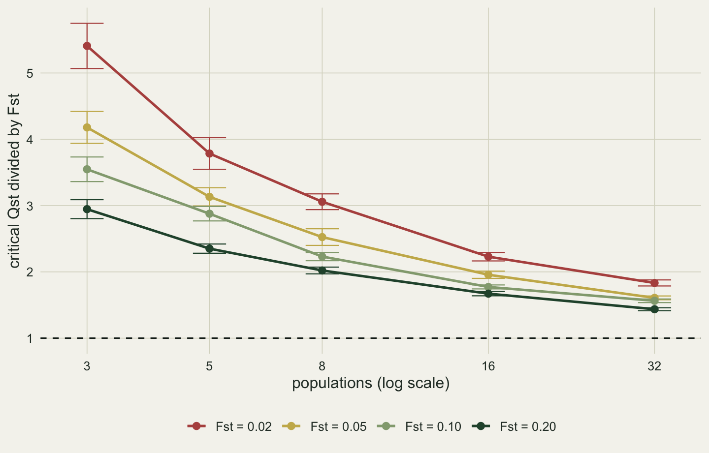
At the marker Fst of 0.10 an estimate has to exceed Fst by a factor of 3.55 at 3 populations (bootstrap standard error 0.09) and 1.56 at 32. At an Fst of 0.02 and 3 populations the factor is 5.41. The threshold depends on Fst and on the number of populations together, which is the measured reason a single rule of thumb cannot serve every study.
A calibrated test holds its false-positive rate by construction, so the question becomes power. Divergent selection is imposed below in the simplest way, by stretching each population’s deviation from the ancestral mean so that the true Qst is a fixed multiple of Fst while the within-population architecture stays as drift left it. That describes an outcome of selection rather than a process, and it is enough to price the test.
n_rep_pw <- 2000
mult_true <- c(3, 5)
set.seed(1105)
pw <- do.call(rbind, lapply(mult_true, function(mm) {
  spread <- sqrt((1 - fst_mark) * mm / (1 - mm * fst_mark))
  do.call(rbind, lapply(seq_along(d_vec), function(i) {
    r <- replicate_qst(d_vec[i], n_sire0, n_off0, fst_mark, n_rep_pw, spread)
    data.frame(true_mult = mm, n_pop = d_vec[i], mean_qst = mean(r[, "qst"]),
               pw_point = mean(r[, "qst"] > fst_mark),
               pw_cal = mean(r[, "qst"] > main$q_crit[i]))
  }))
}))
pw3 <- pw[pw$true_mult == mult_true[1], ]
pw5 <- pw[pw$true_mult == mult_true[2], ]
target_pw <- 0.8pw$label <- factor(sprintf("true Qst = %d x Fst", pw$true_mult))
pw_long <- rbind(
data.frame(pw[, c("n_pop", "label")], power = pw$pw_cal, rule = "calibrated test"),
data.frame(pw[, c("n_pop", "label")], power = pw$pw_point, rule = "Qst > Fst"))
pw_long$se <- mc_se(pw_long$power, n_rep_pw)
ggplot(pw_long, aes(n_pop, power, colour = rule, linetype = label)) +
geom_hline(yintercept = target_pw, colour = te_body, linetype = "dotted") +
geom_errorbar(aes(ymin = power - 2 * se, ymax = power + 2 * se),
width = 0.06, linewidth = 0.4, linetype = "solid") +
geom_line(linewidth = 0.9) + geom_point(size = 2.2) +
scale_x_log10(breaks = d_vec) +
scale_y_continuous(limits = c(0, 1.02)) +
scale_colour_manual(values = c(`calibrated test` = te_forest, `Qst > Fst` = te_rust),
name = NULL) +
scale_linetype_manual(values = c("solid", "22"), name = NULL) +
labs(x = "populations (log scale)", y = "probability of rejecting neutrality") +
theme_book() + theme(legend.box = "vertical")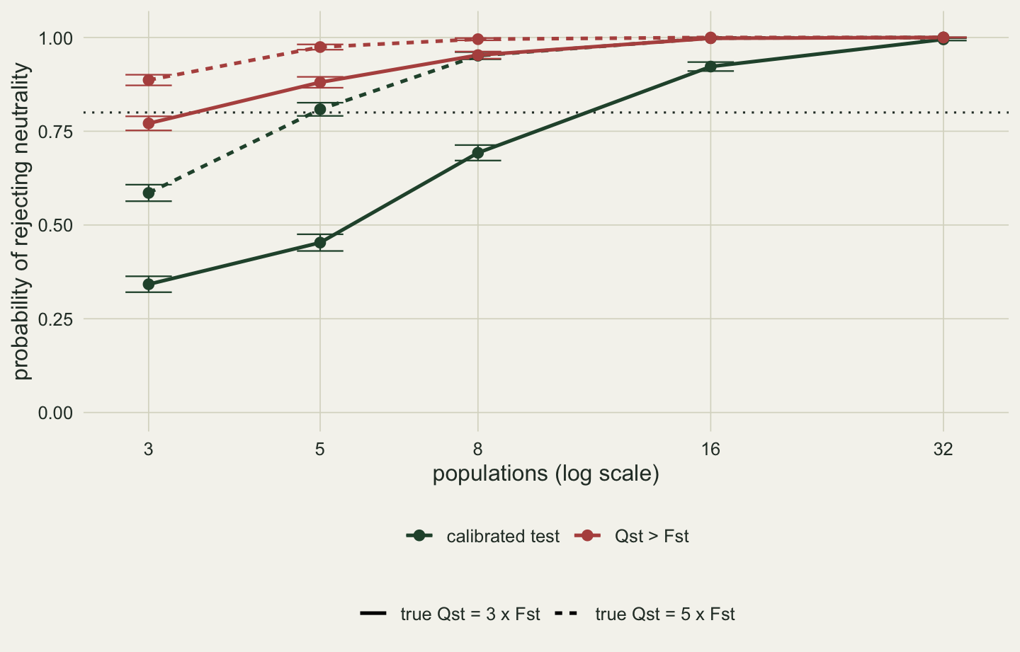
With 3 populations the calibrated test detects a threefold excess in 34 per cent of data sets and a fivefold excess in 59 per cent. The threefold excess needs 16 populations before the power passes 0.80, where it reaches 0.922. The point comparison looks far better on the same figure, 77 per cent for the threefold case at 3 populations, but that is the power of a rule whose false-positive rate is 0.386, and a power bought that way is not power. A study of 3 populations therefore cannot support either conclusion: under the point rule a positive result is close to uninformative, and under the calibrated test a negative result misses 41 per cent of traits that are five times as differentiated as the markers. Merila and Crnokrak (2001) and later Leinonen and colleagues (2013) found that comparisons of this size were common in the published record.
What a proper analysis needs, then, can be said in terms of the quantities measured above. The number of populations is the sample size of the comparison and should be reported first; individuals within populations buy precision on V_A and very little on the decision. The breeding design and the variance components belong in the report alongside the ratio, so that a reader can see whether the among-population term was corrected for the sampling variance of the means; in the smallest design of the sweep, 8.3 per cent of neutral data sets returned a Qst of exactly one because the estimated V_A fell to zero, and 6.2 per cent returned exactly zero, both of which a bare ratio hides. The comparison with Fst should be a critical value from a simulated null for the design and Fst in hand, and a Qst below it means that neutrality was not rejected, which the power figure shows is a much weaker statement than neutrality. O’Hara and Merila (2005) showed that the estimation problems persist even for purely additive traits, and two simplifications here should make the simulated null narrower than a real one. Fst is treated as a known constant when it is itself an estimate from a finite set of loci, and the populations drift independently from one ancestor with no migration, whereas connected or nested populations carry less independent information than their count suggests. Neither effect was measured here, so the critical multiples above are best read as optimistic. A third simplification cuts the other way: dominance, left out of the model, pulls Qst below Fst under drift, which makes the comparison conservative for divergent selection.
11.6 From variance components to exact accounting
Qst against Fst closes Part III on a comparison of two variance ratios, and like everything in Parts II and III it rests on a model: additive loci, a drift process, a breeding design with known expected mean squares. The breeder’s equation, the multivariate response through G and now the neutral theory of divergence all predict how a mean changes, or how far means drift apart, from variances and covariances that the animal model estimates. Chapter 12 steps back from every one of those models. The Price equation writes the change in any mean as a covariance with fitness plus a transmission term, with no assumption about genes, loci or distributions, and each of these predictions turns out to be a special case of it, obtained by saying what the covariance and the transmission term are in that setting.
References
Lande R 1992. Evolution 46(2):381-389 (10.1111/j.1558-5646.1992.tb02046.x)
Spitze K 1993. Genetics 135(2):367-374 (10.1093/genetics/135.2.367)
Merila J, Crnokrak P 2001. Journal of Evolutionary Biology 14(6):892-903 (10.1046/j.1420-9101.2001.00348.x)
O’Hara RB, Merila J 2005. Genetics 171(3):1331-1339 (10.1534/genetics.105.044545)
Whitlock MC 2008. Molecular Ecology 17(8):1885-1896 (10.1111/j.1365-294X.2008.03712.x)
Whitlock MC, Guillaume F 2009. Genetics 183(3):1055-1063 (10.1534/genetics.108.099812)
Leinonen T, McCairns RJS, O’Hara RB, Merila J 2013. Nature Reviews Genetics 14(3):179-190 (10.1038/nrg3395)