sim_pedigree <- function(n_founders, n_gen, n_dams, n_sires, mean_brood) {
  sex  <- rep(c("M", "F"), length.out = n_founders)
  sire <- dam <- gen <- rep(0L, n_founders)
  alive <- seq_len(n_founders); pools <- list()
  for (g in seq_len(n_gen)) {
    males   <- alive[sex[alive] == "M"]
    females <- alive[sex[alive] == "F"]
    dams_g  <- sample(females, min(n_dams, length(females)))
    pools[[g]] <- sample(males, min(n_sires, length(males)))   # this year's breeding males
    sires_g <- sample(pools[[g]], length(dams_g), replace = TRUE)
    brood   <- 1L + rpois(length(dams_g), mean_brood - 1)
    k <- sum(brood)
    sire <- c(sire, rep(sires_g, brood)); dam <- c(dam, rep(dams_g, brood))
    gen  <- c(gen, rep(g, k)); sex <- c(sex, sample(c("M", "F"), k, replace = TRUE))
    alive <- (length(sire) - k + 1L):length(sire)
  }
  list(sire = sire, dam = dam, sex = sex, gen = gen, n = length(sire), pools = pools)
}
build_A <- function(sire, dam) {
  n <- length(sire); A <- matrix(0, n, n)
  for (i in seq_len(n)) {
    s <- sire[i]; d <- dam[i]
    if (i > 1L) {
      j <- seq_len(i - 1L)
      A[i, j] <- A[j, i] <- 0.5 * ((if (s > 0L) A[j, s] else 0) + (if (d > 0L) A[j, d] else 0))
    }
    A[i, i] <- 1 + if (s > 0L && d > 0L) A[s, d] / 2 else 0
  }
  A
}
ped_design <- list(n_founders = 80, n_gen = 4, n_dams = 20, n_sires = 18, mean_brood = 4)
set.seed(7071)
ped <- do.call(sim_pedigree, ped_design)
n_ind <- ped$n
A <- build_A(ped$sire, ped$dam)
male <- as.numeric(ped$sex == "M")
X <- cbind(1, male); one <- matrix(1, n_ind, 1)10 Checking an animal model
Chapter 9 dealt with resemblance that an additive term alone cannot account for. A shared nest makes siblings alike for reasons that have nothing to do with their own alleles, a mother’s phenotype reaches her young and, through her breeding value, the young of her relatives, and the animal model reads either as additive variance whenever it has nowhere else to put it. The cure was structural: a term for the shared environment, a design that lets it be estimated, and fostering to separate the mother who supplies the genes from the mother who supplies the care. That chapter ended on the predicted breeding values such a model hands to a second analysis, and this chapter reaches them last. The failures measured here survive a model with the right random effects. The pedigree can be wrong in a way nobody sees. The heritability is a ratio whose denominator depends on the fixed effects and on where the animals lived. A small estimate sits against a wall at zero that changes both its distribution and its test. And predicted breeding values are routinely taken out of the model and used as data elsewhere, which is where promises made in Chapter 4 and Chapter 2 fall due.
10.1 One pedigree and one fitter
Every check runs on the nest-box pedigree of Chapter 7, drawn again with the same design and seed. The simulator now also records which males bred in each generation, a pool of plausible wrong fathers for the first check.
The fitter is the one of Chapter 8: rotate the phenotypes by the eigenvectors of A, profile out the total variance, and search over h^2 alone. It now also compares the best interior value with the likelihood at exactly zero, so that an estimate can land on the boundary rather than a hair above it, and returns the likelihood ratio statistic against h^2 = 0. Two identities are checked first: at h^2 = 0 the profiled variance must equal the residual mean square of lm(), and elsewhere the rotated likelihood must equal the one computed from the full covariance matrix.
prep <- function(A) {
  eg <- eigen(A, symmetric = TRUE)
  list(d = pmax(eg$values, 1e-9), U = eg$vectors, n = nrow(A))
}
reml_h2 <- function(y, X, st) {
  ys <- drop(crossprod(st$U, y)); Xs <- crossprod(st$U, X)
  n <- st$n; p <- ncol(X)
  core <- function(h2) {
    lam <- h2 * st$d + 1 - h2
    XtHX <- crossprod(Xs, Xs / lam); XtHy <- crossprod(Xs, ys / lam)
    ch <- chol(XtHX); b <- backsolve(ch, forwardsolve(t(ch), XtHy))
    ss <- sum(ys^2 / lam) - sum(XtHy * b)
    list(ll = -0.5 * ((n - p) * log(ss / (n - p)) + sum(log(lam)) + 2 * sum(log(diag(ch)))),
         vp = ss / (n - p), b = drop(b), lam = lam)
  }
  at0 <- core(0)
  op <- optimize(function(h) core(h)$ll, c(0, 0.999), maximum = TRUE, tol = 1e-7)
  h2 <- if (op$objective > at0$ll) op$maximum else 0
  f <- core(h2)
  list(h2 = h2, va = h2 * f$vp, vr = (1 - h2) * f$vp, vp = f$vp, b = f$b, ll = f$ll,
       lrt = max(0, 2 * (f$ll - at0$ll)), ys = ys, Xs = Xs, lam = f$lam)
}
st <- prep(A)
L_A <- st$U %*% diag(sqrt(st$d))
bv <- function(va) drop(L_A %*% rnorm(n_ind)) * sqrt(va)   # breeding values with covariance A va

set.seed(10100)
y_chk <- 10 + 0.5 * male + bv(0.5) + rnorm(n_ind, 0, sqrt(0.5))
gap_ols <- abs(reml_h2(y_chk, X, prep(diag(n_ind)))$vp - summary(lm(y_chk ~ male))$sigma^2)
ll_dense <- function(h2) {
  H <- h2 * A + (1 - h2) * diag(n_ind); Hi <- solve(H); XHX <- t(X) %*% Hi %*% X
  r <- y_chk - X %*% solve(XHX, t(X) %*% Hi %*% y_chk); nm <- n_ind - ncol(X)
  -0.5 * (nm * log(drop(t(r) %*% Hi %*% r) / nm) + determinant(H)$modulus + determinant(XHX)$modulus)
}
ll_rot <- function(h2) {                       # the fitter's core, evaluated at a fixed h2
  f <- reml_h2(y_chk, X, st); lam <- h2 * st$d + 1 - h2
  XHX <- crossprod(f$Xs, f$Xs / lam); XHy <- crossprod(f$Xs, f$ys / lam); nm <- n_ind - ncol(X)
  ss <- sum(f$ys^2 / lam) - drop(crossprod(XHy, solve(XHX, XHy)))
  -0.5 * (nm * log(ss / nm) + sum(log(lam)) + determinant(XHX)$modulus)
}
gap_ll <- max(abs(sapply(c(0.1, 0.4, 0.8), function(h) ll_dense(h) - ll_rot(h))))
stopifnot(gap_ols < 1e-10, gap_ll < 1e-8)
Both identities hold to the precision of the arithmetic. The pedigree has 412 birds with a mean inbreeding coefficient of 0.017, as in Chapter 7.
10.2 Fathers that are not fathers
A field pedigree is wrong in a particular way. The mother is usually right, because someone caught her on the nest. The father is the male seen feeding the chicks, and in many songbirds some of the young were sired by a neighbour. The check below moves a given share of sire links to another male breeding in the same generation, simulates phenotypes on the true pedigree, and fits every data set with both matrices.
The arithmetic most people do in their heads says that if a proportion p of sire links is wrong, h^2 falls to about 1 - p of its true value. The alternative is the textbook result for a predictor measured with error: the coefficient is attenuated by the regression of the true predictor on the recorded one. Here the predictor is relatedness, and that factor can be computed from the two matrices before any phenotype is drawn.
corrupt_sires <- function(ped, p) {
  s <- ped$sire; idx <- which(s > 0L)
  for (i in sample(idx, round(p * length(idx)))) {
    pool <- ped$pools[[ped$gen[i]]]; alt <- pool[pool != s[i]]
    s[i] <- alt[sample.int(length(alt), 1L)]
  }
  s
}
rates <- c(0, 0.1, 0.2, 0.3, 0.4); n_err <- 10; n_phen <- 6
V_A_p <- 0.5; V_R_p <- 0.5
low <- lower.tri(A); a_off <- A[low]
set.seed(10101)
err_res <- do.call(rbind, lapply(rates, function(p) do.call(rbind, lapply(seq_len(n_err), function(e) {
  A_bad <- build_A(corrupt_sires(ped, p), ped$dam); st_bad <- prep(A_bad)
  atten <- cov(a_off, A_bad[low]) / var(A_bad[low])   # errors-in-variables factor
  t(replicate(n_phen, {
    y <- 10 + 0.5 * male + bv(V_A_p) + rnorm(n_ind, 0, sqrt(V_R_p))
    f_bad <- reml_h2(y, X, st_bad); f_ok <- reml_h2(y, X, st)
    c(rate = p, atten = atten, h2_bad = f_bad$h2, h2_ok = f_ok$h2, gap = f_ok$ll - f_bad$ll)
  }))
}))))
err_res <- as.data.frame(err_res)
err_tab <- aggregate(cbind(atten, h2_bad, h2_ok, gap) ~ rate, data = err_res, FUN = mean)
err_tab$se_bad <- tapply(err_res$h2_bad, err_res$rate, sd) / sqrt(n_err * n_phen)
err_tab$ratio  <- err_tab$h2_bad / err_tab$h2_ok
err_tab$gap_gt2 <- tapply(err_res$gap > 2, err_res$rate, mean)
err_tab$bad_wins <- tapply(err_res$gap < 0, err_res$rate, mean)
top <- nrow(err_tab); low_rate <- 2
Measured against the true pedigree on the same data, the estimate falls as the error rate rises, but slowly. At the highest rate, 40 per cent of sire links wrong, the recorded pedigree gives a mean h^2 of 0.385 against 0.510 from the true pedigree on the same data, a ratio of 0.754. The proportional rule predicted 0.60; the attenuation factor of the two matrices is 0.800, and the measured ratio lies close to it. Each rate rests on 10 error patterns with 6 phenotype sets each.
A wrong sire does not erase relationships. He is a breeding male from the same small population, often related to the true father, and every dam link is intact, so the recorded matrix is a noisy copy of the true one rather than a diluted one, and noise attenuates by a factor that has to be computed rather than guessed.
pl <- rbind(
  data.frame(rate = rates, h2 = err_tab$h2_bad, series = "recorded pedigree"),
  data.frame(rate = rates, h2 = err_tab$h2_ok, series = "true pedigree"),
  data.frame(rate = rates, h2 = err_tab$h2_ok * (1 - rates), series = "proportional rule"),
  data.frame(rate = rates, h2 = err_tab$h2_ok * err_tab$atten, series = "attenuation factor"))
pl$series <- factor(pl$series, levels = unique(pl$series))
ggplot(pl, aes(rate, h2, colour = series, linetype = series)) +
  geom_line(linewidth = 0.8) +
  geom_errorbar(data = data.frame(rate = rates, lo = err_tab$h2_bad - err_tab$se_bad,
                                  hi = err_tab$h2_bad + err_tab$se_bad),
                aes(x = rate, ymin = lo, ymax = hi), inherit.aes = FALSE,
                width = 0.01, colour = te_rust) +
  geom_point(size = 2) +
  scale_colour_manual(values = c(te_rust, te_forest, te_gold, te_sage), name = NULL) +
  scale_linetype_manual(values = c("solid", "solid", "dashed", "dashed"), name = NULL) +
  labs(x = "share of sire links that are wrong", y = "heritability estimate") +
  guides(colour = guide_legend(nrow = 2)) +
  theme_book()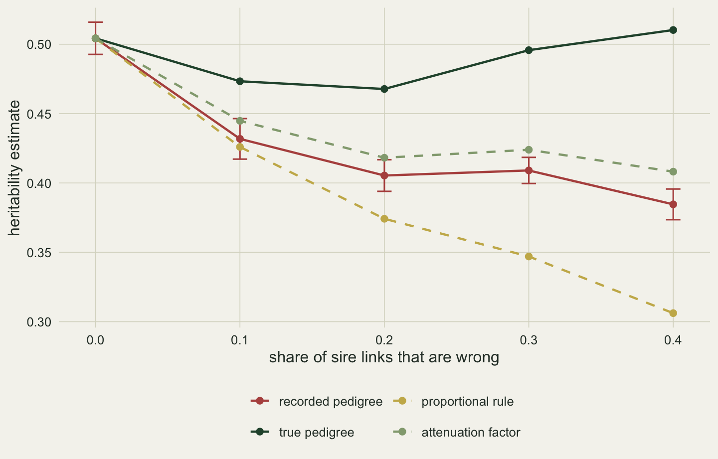
At 10 per cent wrong sires the true pedigree beats the corrupted one by 2.81 log-likelihood units on average, yet the corrupted one fits better in 15 per cent of data sets. In any case a real study has no true pedigree to compare with, and one fitted model says nothing about whether its fathers are right. The check is molecular: genotype a sample of broods, estimate the extra-pair rate, and judge the attenuation that rate implies by simulating sire errors on the pedigree in hand, a calculation on A rather than the subtraction of a proportion; the factor above used the true matrix, which no study has.
10.3 What the ratio is a ratio of
Heritability is V_A / V_P, and arguments about it usually concern the numerator. Comparability more often breaks in the denominator, because the V_P of a fitted animal model is what remains after the fixed effects have taken their share, the problem Chapter 6 met for repeatability. The check below simulates a trait with a sex difference and an environmental covariate and fits it three ways: intercept only, with sex, and with sex and the covariate.
n_rep_d <- 200; male_d <- 2; env_d <- 1.5; V_A_d <- 1; V_R_d <- 1
set.seed(10102)
den <- t(replicate(n_rep_d, {
  envq <- rnorm(n_ind)
  y <- 10 + male_d * male + env_d * envq + bv(V_A_d) + rnorm(n_ind, 0, sqrt(V_R_d))
  fits <- list(reml_h2(y, one, st), reml_h2(y, X, st), reml_h2(y, cbind(X, envq), st))
  c(sapply(fits, `[[`, "h2"), sapply(fits, `[[`, "vp"), sapply(fits, `[[`, "va"))
}))
den_m <- colMeans(den); den_se <- apply(den, 2, sd) / sqrt(n_rep_d)
h2_d <- den_m[1:3]; vp_d <- den_m[4:6]; va_d <- den_m[7:9]; va_se <- den_se[7:9]
With V_A = 1.00 and V_R = 1.00 throughout, three heritabilities come from one generating process: 0.219 with no fixed effects, 0.234 with sex, and 0.492 with sex and the covariate, the last 2.25 times the first. The phenotypic variance falls from 5.29 to 4.26 when sex enters the model and to 2.01 when the covariate follows. Each could be published.
The numerator moved too. The mean additive variance is 1.176 with no fixed effects and 1.011 and 0.997 with them, against the true 1.00, and the first sits 4.2 Monte Carlo standard errors above the truth. Part of the omitted sex effect went to V_A, and how much depends on how the covariate is spread over the pedigree. The chunk below omits, one at a time, the sex vector and fresh coin-flip covariates of the same effect, from a trait with no other fixed effect, and records the shift in V_A. It also predicts each shift in advance: an omitted fixed effect \(\mathbf m\) adds \(\tfrac{1}{2}\mathbf m'\mathbf Q\mathbf A\mathbf Q\mathbf m\) and \(\tfrac{1}{2}\mathbf m'\mathbf Q\mathbf Q\mathbf m\) to the expected REML scores for V_A and V_R, where \(\mathbf Q\) is the REML projection matrix, and the inverse of the information matrix turns those into a first-order shift in the two estimates.
shift_when_omitted <- function(v) mean(replicate(n_rep_probe,
  reml_h2(10 + male_d * v + bv(V_A_d) + rnorm(n_ind, 0, sqrt(V_R_d)), one, st)$va)) - V_A_d
# first-order prediction: an omitted term m adds m'PAPm / 2 and m'PPm / 2 to the expected
# REML scores for V_A and V_R; the inverse information turns that into a shift
V_d <- V_A_d * A + V_R_d * diag(n_ind); Vi_d <- solve(V_d)
P_d <- Vi_d - Vi_d %*% one %*% solve(crossprod(one, Vi_d %*% one), crossprod(one, Vi_d))
PA <- P_d %*% A
info <- 0.5 * matrix(c(sum(PA * t(PA)), sum(PA * t(P_d)), sum(PA * t(P_d)), sum(P_d * t(P_d))), 2)
predicted_shift <- function(v) {
  m <- male_d * v
  solve(info, 0.5 * c(drop(t(m) %*% PA %*% P_d %*% m), drop(t(m) %*% P_d %*% P_d %*% m)))[1]
}
n_probe <- 16; n_rep_probe <- 40
set.seed(10103)
covs <- cbind(sex = male, replicate(n_probe, rbinom(n_ind, 1, 0.5)))
probe <- cbind(pred = apply(covs, 2, predicted_shift), shift = apply(covs, 2, shift_when_omitted))
probe_cor <- cor(probe[, "pred"], probe[, "shift"])
coin <- probe[-1, ]
Leaving the sex vector out of this simpler model raises V_A by +0.468, against a first-order prediction of +0.500. The 16 coin-flip covariates, 40 data sets each, shift it by between -0.138 and +0.199, and over all 17 covariates prediction and measurement correlate at 0.93. The sex vector lies well beyond that range although it carries no genetic information, because the pedigree fixes it for every breeder: all sires are male and all dams female, so sex lines up with the parent-offspring links from which A is built. A covariate can move V_A down as well as up. The shift belongs to the covariate and the pedigree and can be computed before fitting. Coin flips are shared by relatives only by chance; hatch date or natal territory are shared by construction, and their predicted shift is worth computing before they are left out.
There is no single correct denominator. To predict the response to selection as the animals experience it, the variance selection sees belongs in V_P; to compare with a laboratory estimate that removed a covariate by design, it belongs out. What cannot be defended is a ratio without its model. Reporting V_A, V_R and the fixed effects beside h^2 lets a later reader rebuild whichever ratio a comparison needs.
10.4 A ratio that moves with the environment
The denominator also moves with no change to the model, because V_R depends on where the animals live. Chapter 5 measured evolvability as the additive variance along a direction of selection. Houle (1992) proposed a scale that does not divide by V_P at all, the mean-standardised additive variance \(I_A = V_A / \bar z^2\), the expected proportional change in the mean per unit strength of selection; it needs a trait with a natural zero, such as a length or a count. The chunk holds V_A fixed while raising V_R, then fits four traits whose variances imitate a passerine study.
vr_grid <- c(0.5, 2, 8); n_rep_e <- 40; V_A_e <- 1; mu_e <- 10
set.seed(10104)
sweep <- sapply(vr_grid, function(vr) rowMeans(replicate(n_rep_e, {
  y <- mu_e + bv(V_A_e) + rnorm(n_ind, 0, sqrt(vr)); f <- reml_h2(y, one, st)
  c(h2 = f$h2, va = f$va, IA = f$va / mean(y)^2) })))
traits <- data.frame(trait = c("tarsus length", "wing length", "clutch size", "annual fledglings"),
                     mean = c(20, 60, 5, 4), va = c(0.45, 9, 0.30, 0.5), vr = c(0.45, 13.5, 1.2, 4.5))
n_rep_t <- 60
set.seed(10105)
tr <- t(sapply(seq_len(nrow(traits)), function(i) rowMeans(replicate(n_rep_t, {
  y <- traits$mean[i] + bv(traits$va[i]) + rnorm(n_ind, 0, sqrt(traits$vr[i]))
  f <- reml_h2(y, one, st); c(h2 = f$h2, IA = f$va / mean(y)^2) }))))
rank_cor <- cor(rank(-tr[, "h2"]), rank(-tr[, "IA"]))
With V_A held at 1.00, as V_R rises from 0.50 to 8.00, the mean h^2 falls from 0.652 to 0.114, a factor of 5.7, while the additive variance is estimated between 0.956 and 1.077 and I_A between 0.0095 and 0.0109, against a true 0.0100. The same genotypes in a noisier place have a much lower heritability and the same capacity to evolve.
Ranked by h^2 and by I_A, the four traits come out in orders with a rank correlation of -1.00: exactly reversed. Tarsus length has the highest heritability, 0.501, and the lowest evolvability, 0.0011; annual fledglings have the lowest heritability, 0.112, and an evolvability 32 times larger. The input variances imitate the pattern Houle found in real data, so the simulation did not discover it; it shows what the pattern costs. Heritability belongs in a prediction from a selection differential in trait units, evolvability in comparisons across traits and units (Hansen and colleagues 2011), and reporting both costs nothing.
10.5 The boundary at zero
Chapter 7 showed REML estimates piling up at zero, and Chapter 6 that the likelihood ratio test of a variance against zero follows not a chi-squared distribution with one degree of freedom but an equal mixture of it and a point mass at zero (Self and Liang 1987). The check below repeats both on the nest-box pedigree, with a true h^2 of zero and with a small one of the size often reported for behaviour.
n_rep_b <- 600; h2_small <- 0.05; alpha <- 0.05
set.seed(10106)
small <- t(replicate(n_rep_b, {
  f <- reml_h2(10 + bv(h2_small) + rnorm(n_ind, 0, sqrt(1 - h2_small)), one, st)
  c(h2 = f$h2, lrt = f$lrt) }))
set.seed(10107)
lrt0 <- replicate(n_rep_b, reml_h2(10 + rnorm(n_ind), one, st)$lrt)
crit_naive <- qchisq(1 - alpha, 1); crit_mix <- qchisq(1 - 2 * alpha, 1)
b_zero <- mean(small[, "h2"] == 0); b_mean <- mean(small[, "h2"])
b_med <- median(small[, "h2"]); b_nz <- mean(small[small[, "h2"] > 0, "h2"])
b_q90 <- unname(quantile(small[, "h2"], 0.9))
null_zero <- mean(lrt0 == 0)
size_naive <- mean(lrt0 > crit_naive); size_mix <- mean(lrt0 > crit_mix)
pow_naive <- mean(small[, "lrt"] > crit_naive); pow_mix <- mean(small[, "lrt"] > crit_mix)
At a true h^2 of 0.05, 21 per cent of 600 estimates are exactly zero. The mean of all of them is 0.053 and the median 0.042. Here the mean is close to the truth, because the pile at zero and the long tail to the right roughly balance, and the median lies below it. The estimates that did not land on zero average 0.068, and the upper decile is 0.127. A study that returns zero writes a different paper from one that returns a positive value, so a literature filtered by what gets reported keeps the right-hand part of this distribution.
ggplot(data.frame(h2 = small[, "h2"]), aes(h2)) +
  geom_histogram(binwidth = 0.01, boundary = 0, closed = "left",
                 fill = te_forest, colour = te_paper) +
  geom_vline(xintercept = h2_small, colour = te_rust, linetype = "dashed") +
  labs(x = "heritability estimate", y = "data sets") +
  theme_book()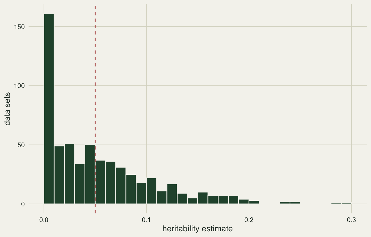
Under a true h^2 of zero the statistic is exactly zero in 56 per cent of data sets, a little more than the half the mixture predicts. At a nominal 5 per cent, the chi-squared reference rejects in 1.5 per cent and the mixture reference in 3.7 per cent, the closer of the two to the nominal level. The naive test is conservative, as it was for repeatability, and the cost is missed heritability: at a true h^2 of 0.05 it detects it in 16 per cent of data sets against 24 per cent for the mixture. The repair is to halve the one-degree-of-freedom p-value and report an interval that may touch zero, naming the reference.
10.6 Predictions used as data
Chapter 4 ended with a remedy for the stasis paradox: estimate the covariance of relative fitness with breeding values, not phenotypes. Chapter 7 produced predicted breeding values and warned that they are narrower than the truth, with errors correlated through the pedigree. The shortcut combines the two, regressing fitness on the predictions, and Postma (2006) and Hadfield and colleagues (2010) showed why it fails. The check below uses the population of Chapter 4, where a bird’s condition raises both its trait and its fitness and has nothing to do with its genes, now on the nest-box pedigree; a second population drops that link and makes fitness heritable, through breeding values independent of the trait’s.
The remedy Wilson and colleagues (2010) recommend is to put the question inside the animal model: fit trait and fitness together, with two-by-two matrices G and E, additive and residual, and read the genetic covariance directly. The rotation by the eigenvectors of A still works, since each rotated contrast carries a pair of values with covariance \(d_i\mathbf G + \mathbf E\), and both matrices are built from Cholesky factors, the device of Chapter 7. The chunk checks the rotated likelihood against the full covariance matrix, and the predictions against the direct formula of Chapter 7.
q1 <- drop(crossprod(st$U, rep(1, n_ind)))
chol2 <- function(t) c(exp(t[1])^2, exp(t[1]) * t[2], t[2]^2 + exp(t[3])^2)  # v11, v12, v22
dev_bi <- function(th, Ys) {
  g <- chol2(th[1:3]); r <- chol2(th[4:6])
  s11 <- st$d * g[1] + r[1]; s12 <- st$d * g[2] + r[2]; s22 <- st$d * g[3] + r[3]
  dt <- s11 * s22 - s12^2; i11 <- s22 / dt; i12 <- -s12 / dt; i22 <- s11 / dt
  M <- matrix(c(sum(q1^2 * i11), sum(q1^2 * i12), sum(q1^2 * i12), sum(q1^2 * i22)), 2)
  m <- c(sum(q1 * (i11 * Ys[, 1] + i12 * Ys[, 2])), sum(q1 * (i12 * Ys[, 1] + i22 * Ys[, 2])))
  b <- solve(M, m); r1 <- Ys[, 1] - q1 * b[1]; r2 <- Ys[, 2] - q1 * b[2]
  sum(log(dt)) + log(det(M)) + sum(i11 * r1^2 + 2 * i12 * r1 * r2 + i22 * r2^2)
}
fit_bi <- function(z, w) {
  Ys <- crossprod(st$U, cbind(z, w)); s <- log(sqrt(c(var(z), var(w)) / 2))
  op <- optim(c(s[1], 0, s[2], s[1], 0, s[2]), dev_bi, Ys = Ys, method = "L-BFGS-B",
              lower = c(-7, -5, -7, -7, -5, -7), upper = c(3, 5, 3, 3, 5, 3),
              control = list(maxit = 1000, factr = 1e5))
  c(G = chol2(op$par[1:3]), R = chol2(op$par[4:6]))
}
blup_of <- function(f) drop(st$U %*% (f$h2 * st$d / f$lam * (f$ys - f$Xs %*% f$b)))

# checks: rotated bivariate deviance against the full matrix, BLUP against V_A A V^-1 (y - Xb)
set.seed(10108)
zc <- rnorm(n_ind); wc <- rnorm(n_ind); th <- c(-0.5, 0.2, -0.7, -0.3, 0.1, -0.4)
Gc <- matrix(chol2(th[1:3])[c(1, 2, 2, 3)], 2); Rc <- matrix(chol2(th[4:6])[c(1, 2, 2, 3)], 2)
Vbig <- kronecker(Gc, A) + kronecker(Rc, diag(n_ind)); Xbig <- kronecker(diag(2), one)
Vi <- solve(Vbig); XVX <- t(Xbig) %*% Vi %*% Xbig
rb <- c(zc, wc) - Xbig %*% solve(XVX, t(Xbig) %*% Vi %*% c(zc, wc))
dev_full <- determinant(Vbig)$modulus + determinant(XVX)$modulus + drop(t(rb) %*% Vi %*% rb)
f_c <- reml_h2(y_chk, X, st)
V_c <- f_c$va * A + f_c$vr * diag(n_ind)
u_direct <- drop(f_c$va * A %*% solve(V_c, y_chk - X %*% f_c$b))
stopifnot(abs(dev_full - dev_bi(th, crossprod(st$U, cbind(zc, wc)))) < 1e-6,
          max(abs(u_direct - blup_of(f_c))) < 1e-8)

z3 <- function(x) f3(ifelse(abs(x) < 5e-4, 0, x))   # no minus sign on a rounded zero
V_A_w <- 0.4; V_R_w <- 0.6; rho_c <- 0.7; V_fit <- 0.3
sim_fitness <- function(route) {
  a <- bv(V_A_w); cond <- rnorm(n_ind)
  z <- a + sqrt(V_R_w) * (rho_c * cond + sqrt(1 - rho_c^2) * rnorm(n_ind))
  eta <- if (route == "condition") 0.2 + 0.4 * cond else 0.2 + bv(V_fit)
  W <- rpois(n_ind, exp(eta)); w <- W / mean(W)
  f <- reml_h2(z, one, st); a_hat <- blup_of(f); bi <- fit_bi(z, w)
  c(S = cov(z, w), h2S = f$h2 * cov(z, w), R_true = cov(a, w), R_blup = cov(a_hat, w),
    p_blup = summary(lm(w ~ a_hat))$coefficients[2, 4],
    G_zw = bi[["G2"]], R_zw = bi[["R2"]])
}
n_rep_w <- 100
set.seed(10109); fc <- t(replicate(n_rep_w, sim_fitness("condition")))
set.seed(10110); fh <- t(replicate(n_rep_w, sim_fitness("heritable")))
mc <- colMeans(fc); mh <- colMeans(fh)
se_c <- apply(fc, 2, sd) / sqrt(n_rep_w); se_h <- apply(fh, 2, sd) / sqrt(n_rep_w)
rej_c <- mean(fc[, "p_blup"] < alpha); rej_h <- mean(fh[, "p_blup"] < alpha)
Both checks pass to the precision of the arithmetic. In the population where condition drives fitness, 100 replicate studies give a mean selection differential of 0.212 and a breeder’s-equation prediction of 0.084, while the true covariance of breeding value with relative fitness averages -0.002 (Monte Carlo standard error 0.003): no response. The covariance of the predicted breeding values with fitness averages 0.064, 75 per cent of the spurious prediction, and the regression of fitness on them is significant at 5 per cent in 81 per cent of studies. Each prediction leans on the bird’s own phenotype, which carries its condition. The bivariate model puts that covariance where it belongs: the residual covariance of trait and fitness averages 0.208, and the genetic covariance 0.004 (standard error 0.006).
In the second population fitness is heritable but genetically unrelated to the trait. The predictions are unbiased there, a mean covariance of 0.002, but the regression treats 412 related birds as independent and rejects a true null in 27 per cent of studies at a nominal 5 per cent. The bivariate genetic covariance averages 0.002 (standard error 0.009). So predicted breeding values carried into a second analysis give a biased answer when an environment links trait and fitness, and an overconfident one even when nothing does.
V_I <- 0.37; V_Rb <- 0.63; s_annual <- 0.55; life_cap <- 10
lrs_year <- 1.2; nb_size <- 1.5; p_later <- 0.6; v_floor <- 0.05; n_anim <- 150
The second promise, made in Chapter 2, concerns a behavioural score and the curvature of selection on it. Suppose each of 150 animals is tested once in its first year and then in each later year it is found alive, with probability 60 per cent, so long-lived animals have more tests and more offspring. With V_I = 0.37 and V_R = 0.63, in the notation of Chapter 6, an animal tested k times has reliability \(k V_I / (k V_I + V_R)\), and its predicted value is its mean deviation shrunk by it. The expected square of the prediction therefore rises with k, while that of the raw mean, \(V_I + V_R / k\), falls. With no selection, the extremes of the predicted scores belong to long-lived, successful animals and a parabola through them opens upward; the extremes of the raw means belong to short-lived animals and it opens downward. The squared prediction plus its prediction error variance has expectation V_I for every k, which gives a calibrated repair; a second repair uses only each animal’s first test, calibrated with variances estimated by moments. Gradients are doubled as in Chapter 2, and the one-way REML fit is checked against nlme::lme.
gen_pop <- function(n, sel = "none", shuffle = FALSE) {
  a <- rnorm(n, 0, sqrt(V_I)); zt <- a / sqrt(V_I)
  years <- pmin(1 + rgeom(n, 1 - s_annual), life_cap)
  k <- 1L + rbinom(n, years - 1, p_later)                  # tests: one per year found alive
  if (shuffle) k <- sample(k)                              # same counts, no link to fate
  mu_W <- lrs_year * years
  if (sel == "fecundity") mu_W <- mu_W * exp(-0.15 * (zt^2 - 1))
  list(a = a, k = k, W = rnbinom(n, size = nb_size, mu = mu_W))
}
reml_ow <- function(y, id, k) {                            # one-way REML, variance ratio profiled
  N <- length(y); ybar <- as.numeric(rowsum(y, id)) / k; ssw <- sum((y - ybar[id])^2)
  dev <- function(ll) {
    lam <- exp(ll); ci <- k / (1 + k * lam); mu <- sum(ci * ybar) / sum(ci)
    (N - 1) * log((ssw + sum(ci * (ybar - mu)^2)) / (N - 1)) + sum(log(1 + k * lam)) + log(sum(ci))
  }
  lam <- exp(optimize(dev, c(-9, 4), tol = 1e-9)$minimum)
  ci <- k / (1 + k * lam); mu <- sum(ci * ybar) / sum(ci)
  vr <- (ssw + sum(ci * (ybar - mu)^2)) / (N - 1); vi <- lam * vr
  list(vi = vi, vr = vr, mu = mu, ybar = ybar,
       blup = k * lam / (1 + k * lam) * (ybar - mu), pev = vi * vr / (vr + k * vi))
}
gam_fit <- function(w, x1, x2) {                           # doubled quadratic gradient, OLS p
  fit <- summary(lm(w ~ x1 + x2))$coefficients
  c(g = 2 * fit[3, 1], p = fit[3, 4])
}
std <- function(x) (x - mean(x)) / sd(x)
one_study <- function(sel = "none", shuffle = FALSE) {
  p <- gen_pop(n_anim, sel, shuffle); id <- rep(seq_len(n_anim), p$k)
  y <- p$a[id] + rnorm(length(id), 0, sqrt(V_Rb)); f <- reml_ow(y, id, p$k)
  w <- p$W / mean(p$W); zb <- std(f$blup); zr <- std(f$ybar)
  y1 <- y[!duplicated(id)]                                 # every animal's first test
  vr1 <- sum((y - f$ybar[id])^2) / (length(y) - n_anim); vi1 <- var(y1) - vr1
  first <- if (vi1 >= v_floor) {
    r1 <- vi1 / (vi1 + vr1); b1 <- r1 * (y1 - mean(y1))
    gam_fit(w, b1 / sqrt(vi1), (b1^2 + vi1 * (1 - r1)) / vi1)
  } else c(g = NA, p = NA)
  c(blup = gam_fit(w, zb, zb^2), raw = gam_fit(w, zr, zr^2),
    cal = gam_fit(w, f$blup / sqrt(f$vi), (f$blup^2 + f$pev) / f$vi),
    first = first, vi = f$vi, cor_kW = cor(p$k, p$W),
    first_true = gam_fit(w, V_I / (V_I + V_Rb) * y1 / sqrt(V_I),
                         ((V_I / (V_I + V_Rb) * y1)^2 + V_I * V_Rb / (V_I + V_Rb)) / V_I)[["g"]])
}

set.seed(10111)
p_chk <- gen_pop(n_anim); id_chk <- rep(seq_len(n_anim), p_chk$k)
y_b <- p_chk$a[id_chk] + rnorm(length(id_chk), 0, sqrt(V_Rb))
f_hand <- reml_ow(y_b, id_chk, p_chk$k)
f_lme <- nlme::lme(y ~ 1, random = ~ 1 | id, data = data.frame(y = y_b, id = factor(id_chk)))
vc_lme <- as.numeric(nlme::VarCorr(f_lme)[, "Variance"])
stopifnot(max(abs(c(f_hand$vi, f_hand$vr) / vc_lme - 1)) < 1e-4,
          max(abs(f_hand$blup - nlme::ranef(f_lme)[, 1])) < 1e-4)

n_rep_a <- 3000
scen <- data.frame(name = c("no selection", "no selection, counts shuffled", "fecundity selection",
                            "fecundity selection, counts shuffled"),
                   sel = c("none", "none", "fecundity", "fecundity"), shuffle = c(FALSE, TRUE, FALSE, TRUE))
runs <- lapply(seq_len(nrow(scen)), function(i) {
  set.seed(10111 + i)
  m <- t(replicate(n_rep_a, one_study(scen$sel[i], scen$shuffle[i])))
  m[m[, "vi"] >= v_floor, ]
})
arms <- c("blup", "raw", "cal", "first")
gtab <- do.call(rbind, lapply(seq_along(runs), function(i) {
  g <- runs[[i]][, paste0(arms, ".g")]
  data.frame(scenario = scen$name[i], arm = arms, g = colMeans(g, na.rm = TRUE),
             se = apply(g, 2, sd, na.rm = TRUE) / sqrt(colSums(!is.na(g))),
             rej = colMeans(runs[[i]][, paste0(arms, ".p")] < alpha, na.rm = TRUE))
}))
gv <- function(s, a, col = "g") gtab[gtab$scenario == s & gtab$arm == a, col]
kept <- sapply(runs, nrow)
cor_kW <- mean(runs[[1]][, "cor_kW"])
first_true <- sapply(runs, function(m) mean(m[, "first_true"]))
set.seed(10120)
big <- gen_pop(2e5, "fecundity"); zt <- big$a / sqrt(V_I)
oracle <- 2 * unname(coef(lm(I(big$W / mean(big$W)) ~ zt + I(zt^2)))[3])
g_lit <- 0.10                          # median absolute quadratic gradient, Kingsolver et al. 2001
The hand-coded fit and lme agree on both variances and on every predicted value. Each scenario runs 3,000 studies of 150 animals, of which at least 2,998 pass a guard that drops studies whose estimated V_I is too small to divide by. Under no selection the correlation between the number of tests and lifetime success averages 0.46.
lab <- c(blup = "predicted value", raw = "raw mean", cal = "calibrated square", first = "first test")
gp <- gtab; gp$arm_f <- factor(lab[gp$arm], levels = rev(lab))
gp$scenario <- factor(gp$scenario, levels = scen$name)
ref <- data.frame(scenario = factor(scen$name, levels = scen$name), g = c(0, 0, oracle, oracle))
ggplot(gp, aes(g, arm_f)) +
  geom_vline(data = ref, aes(xintercept = g), linetype = "dashed", colour = te_ink) +
  geom_errorbar(aes(xmin = g - 2 * se, xmax = g + 2 * se), orientation = "y",
                width = 0, colour = te_sage, linewidth = 0.8) +
  geom_point(aes(colour = arm), size = 2.6, show.legend = FALSE) +
  scale_colour_manual(values = c(blup = te_forest, raw = te_rust, cal = te_gold, first = te_ink)) +
  facet_wrap(~ scenario, ncol = 2) +
  labs(x = "quadratic selection gradient", y = NULL) +
  theme_book()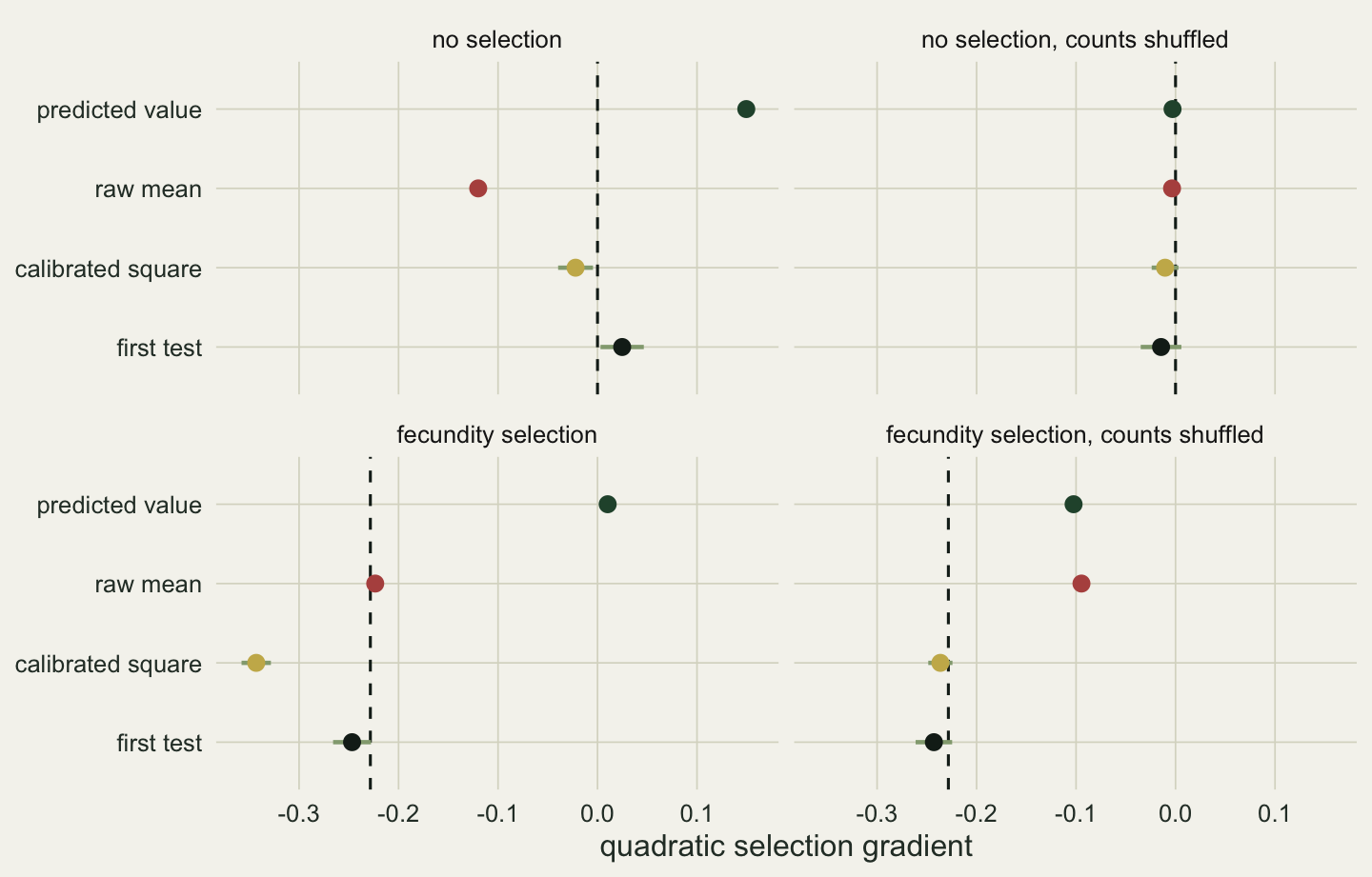
With no selection anywhere, the standardised predicted scores give a mean quadratic gradient of +0.150, apparent disruptive selection, and the standardised raw means -0.120, apparent stabilising selection, from the same studies. The gap between them is 2.69 times the median absolute quadratic gradient of 0.10 compiled by Kingsolver and colleagues (2001). Shuffling the test counts among animals, which keeps the spread of reliabilities but breaks their link with fate, brings every analysis to within 0.015 of zero, so the cause is the link and not the shrinkage. The calibrated square sits at -0.022 (standard error 0.009) and the first test at +0.025 (0.011): small beside the field analyses, though each a couple of standard errors from zero. With the ordinary standard error, a test on the predicted scores rejects a true zero in 20 per cent of studies.
Under real stabilising selection on fecundity, with a true gradient of -0.228, the predicted scores read +0.010: the spurious bowl cancels the real hump. The raw mean reads -0.223. With the counts shuffled under the same selection it reads -0.095, the real curvature diluted by scores averaged over few tests, and that dilution plus the spurious hump of the null scenario gives -0.215. The raw mean lands near the truth because two errors of different origin happen to add up to about the right amount, not because it measures the right thing. The calibrated square overshoots, to -0.343, because the long-lived animals whose calibrated squares vary most also carry most of the offspring and dominate the fit; with the counts shuffled it reads -0.236. The first test, which gives every animal the same precision, reads -0.247 (standard error 0.010); with the true variances in place of the moment estimates the same first tests read -0.241. It lies beyond the truth by 8 per cent of the gradient, 1.9 Monte Carlo standard errors; with the true variances the gap shrinks to 1.3, which these replicates cannot separate from zero. For linear selection Houslay and Wilson (2017) recommend fitting behaviour and fitness in one model, as for breeding values above. That model has no term for curvature. For curvature, a score of equal precision for every animal is the only analysis here that both holds its level, rejecting a true zero in 4.6 per cent of studies, and sizes a real gradient; the calibrated square removes most of the spurious curvature but still rejects a true zero in 10.4 per cent and overshoots real curvature.
10.7 What travels with the number
Each check changed something that would be reported. Wrong fathers lowered the heritability by the attenuation of the relationship matrix, not by the share of wrong links. The fixed effects more than doubled it and moved V_A itself. The environment alone moved it several-fold while the evolvability stayed put. At a small true value the estimate sat exactly on zero in 21 per cent of data sets, and the conventional test missed heritability that was there. And predicted values used as data produced a genetic selection differential out of an environmental covariance and a curvature out of the number of times an animal was tested. None of this argues against the animal model. It argues for reporting with every heritability how fathers were assigned, the fixed effects, the variance components, an interval that can touch zero, and, for anything built on breeding values, a model that estimates the quantity itself rather than a regression on predictions.
All of it concerned variation within one population. Chapter 11 turns to variation among populations, comparing the additive variance between them with the additive variance within them and setting the ratio against the divergence of neutral markers. Every term in that comparison is an animal-model variance of the kind checked here, estimated in populations with different environments, pedigrees and fixed effects, and the checks of this chapter travel with it.
References
Houle D 1992. Genetics 130(1):195-204 (10.1093/genetics/130.1.195)
Hansen TF, Pelabon C, Houle D 2011. Evolutionary Biology 38(3):258-277 (10.1007/s11692-011-9127-6)
Self SG, Liang KY 1987. Journal of the American Statistical Association 82(398):605-610 (10.1080/01621459.1987.10478472)
Postma E 2006. Journal of Evolutionary Biology 19(2):309-320 (10.1111/j.1420-9101.2005.01007.x)
Hadfield JD, Wilson AJ, Garant D, Sheldon BC, Kruuk LEB 2010. The American Naturalist 175(1):116-125 (10.1086/648604)
Wilson AJ, Reale D, Clements MN, Morrissey MM, Postma E, Walling CA, Kruuk LEB, Nussey DH 2010. Journal of Animal Ecology 79(1):13-26 (10.1111/j.1365-2656.2009.01639.x)
Houslay TM, Wilson AJ 2017. Behavioral Ecology 28(4):948-952 (10.1093/beheco/arx023)
Kingsolver JG, Hoekstra HE, Hoekstra JM, Berrigan D, Vignieri SN, Hill CE, Hoang A, Gibert P, Beerli P 2001. The American Naturalist 157(3):245-261 (10.1086/319193)