sim_pedigree <- function(n_founders, n_gen, n_dams, n_sires, mean_brood) {
  sex  <- rep(c("M", "F"), length.out = n_founders)
  sire <- dam <- gen <- rep(0L, n_founders)
  alive <- seq_len(n_founders)
  for (g in seq_len(n_gen)) {
    males   <- alive[sex[alive] == "M"]
    females <- alive[sex[alive] == "F"]
    dams_g  <- sample(females, min(n_dams, length(females)))
    sires_g <- sample(sample(males, min(n_sires, length(males))),
                      length(dams_g), replace = TRUE)   # half sibs via shared sires
    brood   <- 1L + rpois(length(dams_g), mean_brood - 1)
    k <- sum(brood)
    sire <- c(sire, rep(sires_g, brood)); dam <- c(dam, rep(dams_g, brood))
    gen  <- c(gen, rep(g, k)); sex <- c(sex, sample(c("M", "F"), k, replace = TRUE))
    alive <- (length(sire) - k + 1L):length(sire)
  }
  list(sire = sire, dam = dam, sex = sex, gen = gen, n = length(sire))
}
ped_design <- list(n_founders = 80, n_gen = 4, n_dams = 20, n_sires = 18, mean_brood = 4)
set.seed(7071)
ped <- do.call(sim_pedigree, ped_design)
n_ind <- ped$n7 The animal model
Chapter 6 ended with a variance it could not split. Repeated records of the same individual separate what is permanent about an animal from what changes between one measurement and the next, but the permanent part contains two things of very different evolutionary weight: the breeding value, which the animal passes to its offspring, and the permanent environment, the lasting mark of where and how it grew up, which it does not. Measuring the same bird again and again cannot tell them apart, because both follow the bird around. Measuring its relatives can. A daughter inherits on average half of her mother’s breeding value and none of the nest her mother grew up in, so the resemblance between relatives carries the additive variance and leaves the permanent environment behind.
The model that reads resemblance between relatives of every kind at once is the animal model. It is a mixed model with one random effect per individual, whose covariance is not estimated but fixed in advance by the pedigree. This chapter builds it from nothing: the relationship matrix A from a pedigree, a restricted maximum likelihood fit written by hand, the demonstration that the fixed-effect part of that fit is generalised least squares, and the predicted breeding values that come out at the end. It keeps the promise of Chapter 5 that a fitted variance cannot go below zero, and it shows why the predicted breeding values, taken together, are a narrower set of numbers than the breeding values they predict.
7.1 A pedigree and its relationship matrix
A pedigree is a table of three columns: an individual, its sire and its dam, with unknown parents coded as zero and parents listed before their offspring. The simulation below produces one in the shape of a nest-box study of a small, closed bird population. A generation of unrelated founders is followed by several generations in which a limited set of females breed, each with a male drawn with replacement from a smaller set of males, so that some males father several broods and half-sib families appear alongside full-sib ones.
The pedigree holds 412 birds, 80 of them founders, over 4 generations after the founders, with 20 breeding females and at most 18 breeding males in each.
The additive relationship matrix A holds, for every pair of individuals, twice their coefficient of kinship: the expected proportion of their alleles that are identical by descent, counted so that an individual’s relationship with itself is one plus its inbreeding coefficient. Henderson’s tabular method fills it in one pass down the pedigree. For individual \(i\) with sire \(s\) and dam \(d\), and any individual \(j\) listed before it,
\[ A_{ij} = \tfrac{1}{2}\left(A_{js} + A_{jd}\right), \qquad A_{ii} = 1 + \tfrac{1}{2}A_{sd}, \]
with an unknown parent contributing nothing. Because parents come first, everything on the right is known by the time it is needed.
build_A <- function(sire, dam) {
  n <- length(sire); A <- matrix(0, n, n)
  for (i in seq_len(n)) {
    s <- sire[i]; d <- dam[i]
    if (i > 1L) for (j in seq_len(i - 1L)) {
      A[i, j] <- A[j, i] <- (if (s > 0L) A[j, s] / 2 else 0) + (if (d > 0L) A[j, d] / 2 else 0)
    }
    A[i, i] <- 1 + if (s > 0L && d > 0L) A[s, d] / 2 else 0
  }
  A
}
A <- build_A(ped$sire, ped$dam)
F_inb <- diag(A) - 1
min_eig_A <- min(eigen(A, symmetric = TRUE, only.values = TRUE)$values)

# pair classes
up <- upper.tri(A)
known <- ped$sire > 0L
full_sib <- outer(paste(ped$sire, ped$dam), paste(ped$sire, ped$dam), "==") & outer(known, known, "&")
half_sib <- outer(ped$sire, ped$sire, "==") & outer(ped$dam, ped$dam, "!=") & outer(known, known, "&")
g1 <- outer(ped$gen == 1L, ped$gen == 1L, "&")
fs_g1 <- A[full_sib & up & g1]; hs_g1 <- A[half_sib & up & g1]
stopifnot(all(abs(fs_g1 - 0.5) < 1e-12), all(abs(hs_g1 - 0.25) < 1e-12))
fs_all <- A[full_sib & up]
fs_exact <- mean(abs(fs_all - 0.5) < 1e-12)
In the first generation, bred from unrelated founders, the rule gives the textbook values exactly: every full-sib pair sits at 0.50 and every half-sib pair at 0.25, which the code checks rather than trusts. Across the whole pedigree the picture changes. Of 639 full-sib pairs only 69 per cent sit at exactly one half; the mean is 0.523 and the largest 0.750. The mean inbreeding coefficient is 0.017, and 26 per cent of birds are inbred to some degree. Nothing is wrong with the matrix. The textbook values assume that the parents are unrelated and not inbred, and in a closed population of this size that assumption fails within the few generations simulated here: full sibs whose parents are cousins share more than half their additive variation. A sib analysis that groups birds into families and assigns every pair the textbook value discards exactly this information, and the animal model uses it. The smallest eigenvalue of A is 0.071, so the matrix is positive definite and can serve as a covariance matrix.
7.2 The model
The animal model writes the phenotype of each individual as fixed effects plus its breeding value plus a residual,
\[ \mathbf y = \mathbf X \mathbf b + \mathbf Z \mathbf a + \mathbf e, \qquad \mathbf a \sim N(\mathbf 0, \mathbf A V_A), \qquad \mathbf e \sim N(\mathbf 0, \mathbf I V_R), \]
so that the phenotypes have covariance \(\mathbf V = \mathbf Z \mathbf A \mathbf Z' V_A + \mathbf I V_R\). The breeding values are the random effects, and the one thing that distinguishes this from any other mixed model is that their correlation structure is A, known from the pedigree before any phenotype is seen. Only its scale, V_A, is estimated. With one record per bird the residual V_R, the V_E of Chapter 4, holds all non-additive variation, the permanent environment of Chapter 6 included; with repeated records a second individual-level effect with identity covariance takes the permanent environment out of the residual, and the two chapters combine into one model.
To simulate breeding values with covariance exactly A V_A, each individual receives the mean of its parents’ breeding values plus a Mendelian sampling deviation, the chance of which half of each parent’s genome it inherited. That deviation has variance \(\tfrac{1}{2}V_A\left(1 - \tfrac{1}{2}(F_s + F_d)\right)\) when both parents are known: inbred parents are more homozygous and give their offspring less to sample. Written as matrices, the recursion is \(\mathbf a = (\mathbf I - \mathbf T)^{-1}\mathbf m\), with \(\mathbf T\) holding the halves that link offspring to parents and \(\mathbf m\) the Mendelian deviations with diagonal variance \(\mathbf D V_A\). Henderson (1976) used the resulting factorisation \(\mathbf A = (\mathbf I - \mathbf T)^{-1}\mathbf D (\mathbf I - \mathbf T)^{-\prime}\) to write down the inverse of A directly from a pedigree, and it is checked here before any data are drawn.
Pm <- matrix(0, n_ind, n_ind)
Pm[cbind(which(ped$sire > 0), ped$sire[ped$sire > 0])] <- 0.5
Pm[cbind(which(ped$dam > 0),  ped$dam[ped$dam > 0])]   <- 0.5
F_par <- function(p) ifelse(p > 0, F_inb[pmax(p, 1)], -1)   # -1 codes an unknown parent
Dm <- 1 - 0.25 * ((1 + F_par(ped$sire)) + (1 + F_par(ped$dam)))
Linv <- solve(diag(n_ind) - Pm)
stopifnot(max(abs(Linv %*% diag(Dm) %*% t(Linv) - A)) < 1e-10)

V_A <- 0.36; V_R <- 0.64; mu <- 19.5; male_eff <- 0.45
set.seed(7072)
a_true <- drop(Linv %*% rnorm(n_ind, 0, sqrt(Dm * V_A)))
male <- as.numeric(ped$sex == "M")
X <- cbind(1, male)
y <- mu + male_eff * male + a_true + rnorm(n_ind, 0, sqrt(V_R))
The simulated trait is a wing length in millimetres with V_A = 0.36 and V_R = 0.64, so h^2 = 0.36, and males are 0.45 mm longer than females, a fixed effect that the model has to estimate alongside the variances.
7.3 REML written out
Restricted maximum likelihood, from Patterson and Thompson (1971), estimates the variance components from the part of the data that the fixed effects cannot absorb. Its log-likelihood is
\[ \ell_R = -\tfrac{1}{2}\left(\log|\mathbf V| + \log|\mathbf X'\mathbf V^{-1}\mathbf X| + (\mathbf y - \mathbf X\hat{\mathbf b})'\mathbf V^{-1}(\mathbf y - \mathbf X\hat{\mathbf b})\right), \qquad \hat{\mathbf b} = (\mathbf X'\mathbf V^{-1}\mathbf X)^{-1}\mathbf X'\mathbf V^{-1}\mathbf y . \]
The middle term is what makes it restricted: it charges the likelihood for the degrees of freedom spent on estimating b, which is why REML avoids most of the downward bias that ordinary maximum likelihood shows when there are many fixed effects. The fixed effects are profiled out, so the optimiser sees only the two variances. Every bird has a record here, so Z is the identity, and one eigen decomposition of A turns every later determinant and inverse into sums and divisions over its eigenvalues. The variances are optimised on the log scale.
reml_setup <- function(y, X, K) {
  eg <- eigen(K, symmetric = TRUE)
  list(lam = eg$values, Q = eg$vectors, ys = drop(crossprod(eg$vectors, y)),
       Xs = crossprod(eg$vectors, X), y = y, X = X, K = K)
}
neg_ll <- function(par, s) {                    # par = log(V_A), log(V_R)
  dv <- s$lam * exp(par[1]) + exp(par[2])
  XtVi <- t(s$Xs / dv)
  ch <- chol(XtVi %*% s$Xs)
  b <- backsolve(ch, forwardsolve(t(ch), XtVi %*% s$ys))
  r <- s$ys - s$Xs %*% b
  0.5 * (sum(log(dv)) + 2 * sum(log(diag(ch))) + sum(r^2 / dv))
}
reml_fit <- function(s, start = c(0.5, 0.5)) {
  op <- optim(log(start), neg_ll, s = s, control = list(reltol = 1e-12, maxit = 4000))
  op <- optim(op$par, neg_ll, s = s, control = list(reltol = 1e-12, maxit = 4000))
  v <- exp(op$par); dv <- s$lam * v[1] + v[2]
  XtVi <- t(s$Xs / dv)
  list(V_A = v[1], V_R = v[2], h2 = v[1] / sum(v), logL = -op$value,
       b = drop(solve(XtVi %*% s$Xs, XtVi %*% s$ys)))
}
s_wing <- reml_setup(y, X, A)
fit <- reml_fit(s_wing)
The fit returns V_A = 0.336 against a true 0.36, V_R = 0.754 against 0.64, and h^2 = 0.308 against 0.36. The intercept is 19.52 mm and the male effect 0.316 mm, against 19.50 and 0.45.
Whether an additive variance of 0.336 counts as close to 0.36 depends on how sharply the data pin it down, and the likelihood itself answers that. Profiling the restricted log-likelihood over V_A, maximising over V_R at each value, draws the curve in the left panel of the profile figure two sections below.
profile_VA <- function(s, grid) vapply(grid, function(v)
  -optimize(function(le) neg_ll(c(log(v), le), s), c(-8, 3), tol = 1e-10)$objective, 0)
grid_wing <- seq(0.005, 1, length.out = 120)
prof_wing <- profile_VA(s_wing, grid_wing)
drop_95 <- qchisq(0.95, 1) / 2
inside <- grid_wing[prof_wing > fit$logL - drop_95]
supp <- range(inside)
grid_r <- seq(0.3, 1.3, length.out = 120)
prof_r <- vapply(grid_r, function(v)
  -optimize(function(la) neg_ll(c(la, log(v)), s_wing), c(-8, 3), tol = 1e-10)$objective, 0)
supp_r <- range(grid_r[prof_r > fit$logL - drop_95])
rel_w_A <- diff(supp) / fit$V_A; rel_w_R <- diff(supp_r) / fit$V_R
A drop of 1.92 log-likelihood units from the peak, the conventional support limit, spans additive variances from 0.147 to 0.624 on this grid. The interval reaches 0.188 below the estimate and 0.288 above it. The curve falls steeply towards zero and slowly towards large values, which is why the sampling distribution of an additive variance is skewed and a symmetric standard error describes it poorly. The residual variance is better determined: its support interval, from 0.569 to 0.947, spans a width of 50 per cent of the estimate, against 142 per cent for the additive variance. The residual is informed by the whole spread of the data, the additive variance only by how much more alike related birds are than unrelated ones.
7.4 The fixed effects are generalised least squares
Nothing in reml_fit mentions pedigrees. It takes a response, a design matrix and a symmetric positive definite matrix, and the pedigree enters only as that matrix. Given the fitted V, the fixed effects it returns should be exactly the generalised least squares estimate, and the restricted log-likelihood it maximises should be exactly the one a direct implementation computes by inverting V in full. Both claims are checked below against code that shares nothing with reml_fit: it builds V densely, inverts it with solve, and uses a different parameterisation, the total variance and h^2.
V_hat <- A * fit$V_A + diag(n_ind) * fit$V_R
Vi <- solve(V_hat)
b_gls <- drop(solve(t(X) %*% Vi %*% X, t(X) %*% Vi %*% y))
gap_b <- max(abs(b_gls - fit$b))
stopifnot(gap_b < 1e-8)

reml_dense <- function(V_P, h2) {
  V <- V_P * (h2 * A + (1 - h2) * diag(n_ind)); Vi <- solve(V)
  XtViX <- t(X) %*% Vi %*% X
  r <- y - X %*% solve(XtViX, t(X) %*% Vi %*% y)
  -0.5 * (determinant(V)$modulus + determinant(XtViX)$modulus + drop(t(r) %*% Vi %*% r))
}
chk <- expand.grid(V_P = seq(0.6, 1.6, length.out = 5), h2 = seq(0.05, 0.9, length.out = 5))
gap_ll <- max(abs(mapply(function(vp, h) reml_dense(vp, h) +
                           neg_ll(log(c(vp * h, vp * (1 - h))), s_wing), chk$V_P, chk$h2)))
stopifnot(gap_ll < 1e-7)
The two sets of fixed effects agree to the precision of the arithmetic, and so do the two log-likelihoods at all 25 points of a grid spread over the parameter space. The animal model’s fixed effects are the generalised least squares estimate at the fitted covariance matrix, and what REML adds to generalised least squares is an estimate of that matrix’s scale. The consequence reaches beyond pedigrees. Put a phylogenetic covariance matrix in the slot where A sits and the same function fits phylogenetic generalised least squares, with h^2 playing the part of Pagel’s lambda on a tree scaled to unit height (Freckleton and colleagues 2002); with the matrix that marks which records belong to the same individual in that slot, the model becomes the repeatability model of Chapter 6. Whatever goes wrong in one of these models, from a badly conditioned matrix to a variance at its boundary, goes wrong in all of them.
7.5 A variance that cannot go below zero
Chapter 5 found that an unconstrained estimate of G from parent-offspring covariances often had a negative eigenvalue, an additive variance below zero along some combination of traits. The same happens to a single trait when a moment estimator meets a trait with little or no additive variance, and it is worth seeing what the REML fit does instead. The simulation below puts a trait with no additive variance at all on the same pedigree many times, and estimates its heritability twice: by regressing offspring on the mean of their parents, whose slope estimates h^2 directly, and by the REML fit.
n_null <- 200
nf <- ped$sire > 0
set.seed(7073)
null_fits <- t(replicate(n_null, {
  y0 <- mu + male_eff * male + rnorm(n_ind, 0, 1)
  mid <- (y0[ped$sire[nf]] + y0[ped$dam[nf]]) / 2
  f0 <- reml_fit(reml_setup(y0, X, A), start = c(0.2, 0.8))
  c(po = unname(coef(lm(y0[nf] ~ mid))[2]), reml = f0$h2)
}))
po_neg <- mean(null_fits[, "po"] < 0)
reml_zero <- mean(null_fits[, "reml"] < 1e-3)
reml_min <- min(null_fits[, "reml"])
Across 200 simulated traits with a true heritability of zero, the parent-offspring estimate is negative in 54 per cent of cases, close to the half expected of an estimator centred on zero. The REML estimate is never negative: its smallest value is zero to the precision of the optimiser, and in 60 per cent of cases it sits at the boundary, below one part in a thousand of the phenotypic variance. The price is a small upward bias, a mean estimate of 0.016 where the truth is zero, because the estimates that would have been negative are piled at zero instead.
The guarantee is not a property of the REML likelihood itself, which can be evaluated at a negative V_A as long as V stays positive definite. It comes from the parameter space the fit searches, here the logarithms of the variances. With several traits the same device parameterises G through a Cholesky factor L, with \(\mathbf G = \mathbf L \mathbf L'\), and a matrix built that way has no negative eigenvalue whatever L is. That is how multivariate REML fits keep G a valid covariance matrix, and why an eigenvalue of an estimated G sitting at exactly zero is a boundary estimate to be reported as such, not evidence that the variance is truly absent.
pick <- which(null_fits[, "po"] < 0 & null_fits[, "reml"] < 1e-3)[1]
set.seed(7073)
for (k in seq_len(pick)) y_pick <- mu + male_eff * male + rnorm(n_ind, 0, 1)  # that replicate's trait
s_null <- reml_setup(y_pick, X, A)
grid_null <- seq(0.0005, 0.4, length.out = 120)
prof_null <- profile_VA(s_null, grid_null)
stopifnot(which.max(prof_null) == 1L)
The right panel of the figure below shows one of those null traits, chosen as the first replicate whose parent-offspring estimate was negative and whose REML estimate sat at the boundary. Its profile likelihood falls all the way from the lowest additive variance on the grid, so the peak lies at or beyond the boundary, and the fit stops there.
prof_df <- rbind(
  data.frame(v = grid_wing, ll = prof_wing - max(prof_wing), panel = "wing length"),
  data.frame(v = grid_null, ll = prof_null - max(prof_null), panel = "no additive variance"))
prof_df$panel <- factor(prof_df$panel, levels = c("wing length", "no additive variance"))
vl <- data.frame(panel = factor("wing length", levels = levels(prof_df$panel)),
                 x = c(fit$V_A, V_A), what = c("REML estimate", "true value"))
ggplot(prof_df, aes(v, ll)) +
  geom_hline(yintercept = -drop_95, colour = te_line, linewidth = 2) +
  geom_line(colour = te_forest, linewidth = 0.9) +
  geom_vline(data = vl, aes(xintercept = x, linetype = what), colour = te_rust) +
  scale_linetype_manual(values = c("REML estimate" = "dashed", "true value" = "dotted"), name = NULL) +
  facet_wrap(~ panel, scales = "free_x") +
  coord_cartesian(ylim = c(-6, 0.2)) +
  labs(x = "additive genetic variance", y = "restricted log-likelihood (from maximum)") +
  theme_book()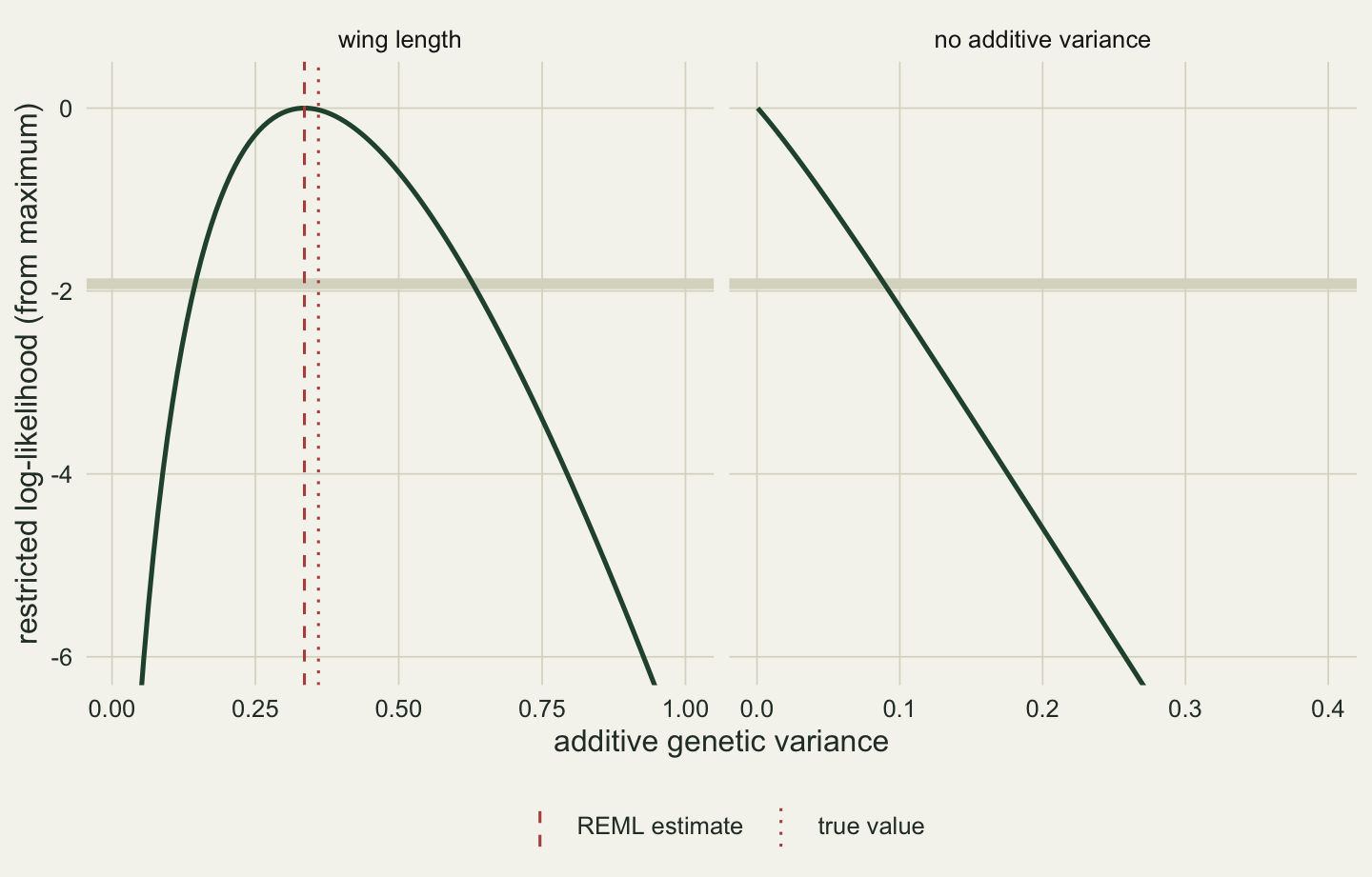
7.6 Breeding values are predictions
With the variances fixed at their estimates, each bird’s breeding value is predicted by the best linear unbiased predictor,
\[ \hat{\mathbf a} = \mathbf A \hat V_A \mathbf V^{-1}(\mathbf y - \mathbf X \hat{\mathbf b}), \]
which takes each bird’s deviation from the fitted fixed effects, weights it by the share of that deviation the additive covariance can explain, and spreads it through A to every relative. Henderson reached the same predictions without ever forming V, by solving the mixed model equations, a system that needs the inverse of A in place of the inverse of V. That inverse is cheap and sparse because of the factorisation checked earlier, and it is what makes animal models on pedigrees of many thousands feasible. Both routes are computed below and compared.
u_hat <- drop(fit$V_A * A %*% Vi %*% (y - X %*% fit$b))
Ainv <- t(diag(n_ind) - Pm) %*% diag(1 / Dm) %*% (diag(n_ind) - Pm)
lhs <- rbind(cbind(crossprod(X), t(X)),
             cbind(X, diag(n_ind) + Ainv * fit$V_R / fit$V_A))
sol <- solve(lhs, c(crossprod(X, y), y))
gap_mme <- max(abs(sol[-(1:2)] - u_hat), abs(sol[1:2] - fit$b))
stopifnot(gap_mme < 1e-8)

XtVi <- t(X) %*% Vi
Pproj <- Vi - t(XtVi) %*% solve(XtVi %*% X, XtVi)
pev <- diag(fit$V_A * A - fit$V_A^2 * A %*% Pproj %*% A)
rel <- 1 - pev / (fit$V_A * diag(A))
n_kin <- rowSums(A >= 0.25) - 1

slope_pt <- cov(u_hat, a_true) / var(a_true)
slope_tp <- cov(u_hat, a_true) / var(u_hat)
sd_ratio <- sd(u_hat) / sd(a_true)
sd_expect <- sqrt(fit$V_A * mean(diag(A) * rel))
terc <- cut(rel, quantile(rel, c(0, 1/3, 2/3, 1)), include.lowest = TRUE,
            labels = c("low", "middle", "high"))
sd_terc <- tapply(u_hat, terc, sd)
cor_terc <- sapply(split(seq_len(n_ind), terc), function(i) cor(u_hat[i], a_true[i]))
The mixed model equations and the direct formula give the same predictions and the same fixed effects to the precision of the arithmetic. The predictions correlate with the true breeding values at 0.685. Each prediction also comes with a prediction error variance, and one minus that variance as a share of the prior variance \(A_{ii} V_A\) is the reliability of the prediction. Reliability averages 0.465 and depends on how much of the pedigree around a bird has been measured: its correlation with the number of relatives at a relationship of a quarter or more is 0.850.
The predictions are spread less widely than the truth. Their standard deviation is 0.385 against 0.568 for the true breeding values, a ratio of 0.678. This is shrinkage, and it follows from the formula: the variance of a bird’s prediction is its prior variance multiplied by its reliability \(\rho_i\), so the expected spread of the whole set is \(\sqrt{\hat V_A \,\overline{A_{ii} \rho_i}}\), which here is 0.399, close to the observed 0.385. Birds with little information are pulled furthest towards zero: in the lowest tercile of reliability the predictions have a standard deviation of 0.361 and correlate with the truth at 0.596, against 0.411 and 0.777 in the highest.
sh <- data.frame(true = a_true, pred = u_hat, rel = terc)
ggplot(sh, aes(true, pred, colour = rel)) +
  geom_abline(slope = 1, intercept = 0, linetype = "dashed", colour = te_ink) +
  geom_abline(slope = slope_pt, intercept = mean(u_hat) - slope_pt * mean(a_true),
              colour = te_ink, linewidth = 0.8) +
  geom_point(size = 1.4, alpha = 0.8) +
  scale_colour_manual(values = c(low = te_gold, middle = te_sage, high = te_rust),
                      name = "reliability tercile") +
  coord_cartesian(ylim = range(a_true)) +
  labs(x = "true breeding value (mm)", y = "predicted breeding value (mm)") +
  theme_book()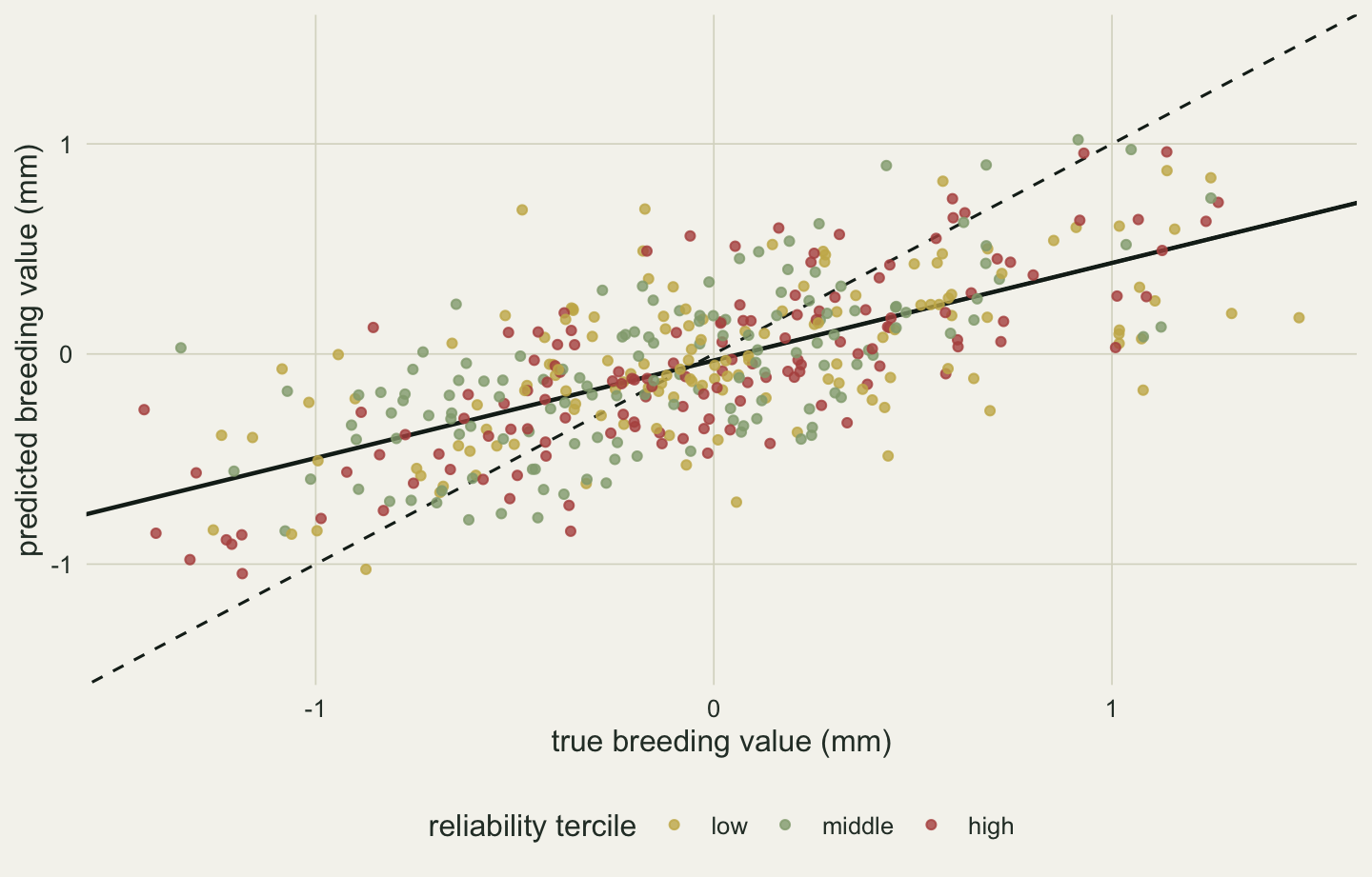
The two regressions between prediction and truth make the point exactly. Prediction regressed on truth has a slope of 0.464, which is the shrinkage visible in the figure. Truth regressed on prediction has a slope of 1.010. The second slope is the one that describes a single prediction, and for BLUP with the true variances its expected value is one: given what the pedigree and the phenotypes say, a bird’s expected breeding value is its prediction, neither too small nor too large. What is too small is the variance of the set. Each prediction is as good a guess as the data allow, and the collection of best guesses is narrower than the collection of true values, because every guess has been drawn towards the mean in proportion to how little is known about it.
That distinction sets up a misuse that is common enough to have its own literature (Hadfield and colleagues 2010). Take the predicted breeding values off the vertical axis of that figure and use them as data in a second analysis, a regression on year to test for genetic change, or a regression of fitness on predicted breeding value to estimate selection on the genes, the shortcut Chapter 4 warned about. The second analysis receives numbers whose spread is too small, whose shrinkage differs from bird to bird with reliability, and whose errors are correlated through the pedigree, and it treats them as independent measurements. Chapter 10 measures what that does to the answer; the remedy there, as Wilson and colleagues (2010) recommend, is to put the question inside the animal model rather than downstream of it.
7.7 How far one pedigree wanders
The estimate of h^2 from this pedigree was 0.308. Whether that is a good answer depends on how much a different pedigree of the same design would have given, and the only way to know is to draw more.
n_rep <- 40
set.seed(7074)
reps <- t(replicate(n_rep, {
  pr <- do.call(sim_pedigree, ped_design)
  Ar <- build_A(pr$sire, pr$dam)
  ar <- drop(t(chol(Ar)) %*% rnorm(pr$n, 0, sqrt(V_A)))
  mr <- as.numeric(pr$sex == "M")
  yr <- mu + male_eff * mr + ar + rnorm(pr$n, 0, sqrt(V_R))
  c(n = pr$n, h2 = reml_fit(reml_setup(yr, cbind(1, mr), Ar))$h2)
}))
h2_true <- V_A / (V_A + V_R)
h2_q <- quantile(reps[, "h2"], c(0.1, 0.9))
Across 40 fresh pedigrees of the same design, averaging 399 birds each, the mean estimate of h^2 is 0.371 against a true 0.36, with a standard deviation of 0.095. The estimates run from 0.204 to 0.529, and the middle eight in ten lie between 0.246 and 0.493. With 40 replicates these spreads are themselves only approximate, but the scale is clear. Two studies of the same population design reporting heritabilities at the two ends of that range would not be in conflict and would not need an ecological explanation for the difference; they would be two draws from one sampling distribution. A pedigree of a few hundred birds supports the statement that wing length is moderately heritable and not much more.
7.8 From one pedigree to many
The animal model has three parts, and each has now been written out and checked. A recursive rule turns the pedigree into A, a matrix that departs from the textbook values as soon as relatives breed with relatives. A restricted likelihood estimates the scale of that matrix and of the residual, keeps both variances non-negative because of the space it searches, and reduces to generalised least squares for the fixed effects. A linear predictor spreads each bird’s deviation across its relatives and returns breeding values that are each well calibrated and together too narrow.
What the chapter has not asked is where the information came from. The pedigree held full sibs, half sibs, parents and offspring, and more distant kin, and the reliability of each prediction rose with the number of close relatives a bird had. Those relatives are not interchangeable. Some contrasts carry much more information about V_A than others, and some carry it at the cost of confounding it with environments that relatives share. Chapter 8 takes the pedigree apart by kind of relative and asks which of them the precision of an animal model depends on.
References
Henderson CR 1976. Biometrics 32(1):69-83 (10.2307/2529339)
Patterson HD, Thompson R 1971. Biometrika 58(3):545-554 (10.1093/biomet/58.3.545)
Freckleton RP, Harvey PH, Pagel M 2002. The American Naturalist 160(6):712-726 (10.1086/343873)
Hadfield JD, Wilson AJ, Garant D, Sheldon BC, Kruuk LEB 2010. The American Naturalist 175(1):116-125 (10.1086/648604)
Wilson AJ, Reale D, Clements MN, Morrissey MM, Postma E, Walling CA, Kruuk LEB, Nussey DH 2010. Journal of Animal Ecology 79(1):13-26 (10.1111/j.1365-2656.2009.01639.x)